 The Climate Change Challenge evaluated publicly available data on climate change and its effects in the Arctic Sea Basin. Nine sub-challenges were set for which parameters were selected, these focused (among others) temperature, ice and phytoplankton. Links to the sub-challenges can be found below.
During the data collection several things came to light. For some topics, such as sea-ice extent for example, a lot of data from different sources was available. For other topics, such as phytoplankton, it can be quite difficult to gather useful data for the entire area. For many parameters, data can be found on a very small spatial and temporal scale, making it difficult to present an overview of the entire Sea Basin. For certain parameters, this also would not make sense as different parts of the sea basin can have completely different circumstances. This was the case not only for phytoplankton, but also for animal behaviour for example. Some practical problems we came across with some examples:
- Data was asked from SAHFOS, this data was freely available for non-profit research scientists but not for commercial enterprises.
- For phytoplankton a collection of data was available on the COPEPOD website, however the data did not cover the entire Sea Basin or the required time period and the data was presented in a format which needed processing before it can be presented in the preferred way.
- Data on Sea Ice was available through a portal of NERSC, however the catalogue had quite technical terms which might confuse non-experts or layman, the same went for the used format in which the data can be downloaded, as this was not a standard format for many data users.
The nine sub-challenges for this challenge were:
Temperature
Sub-challenge: Change in average temperature at surface, 500 meter depth and bottom on a grid over the past 10 years and 50 years.
Results
Historical Arctic data from more than a few decades ago is very different to modern data due to the changes in sampling methods (e.g. the invention of the CTD and initiation of polar orbiting satellites) and differences in sample locations (from individual expeditions to full polar coverage). Archival data is increasingly being merged into digital forms so that historical conditions can be reconstructed. Older data is becoming more available as more reanalysis data sets become available. As more historical data become available in digital forms, we expect reanalyses to become available as well. For now however, the older data should be viewed with care.
This challenge was to find data showing the change in average temperature for the surface (z=0m), 500m depth and bottom over the previous (editor's note: this project finished in 2018) 10 and 50 years on a grid for the entire study area. This practically gave us six different scenarios:
- Change in average temperature for the surface (z=0m) over 10 years on a grid for the entire study area;
- Change in average temperature for 500m depth over 10 years on a grid for the entire study area;
- Change in average temperature for the bottom over 10 years on a grid for the entire study area;
- Change in average temperature for the surface (z=0m) over 50 years on a grid for the entire study area;
- Change in average temperature for 500m depth over 50 years on a grid for the entire study area;
- Change in average temperature for the bottom over 50 years on a grid for the entire study area.
We began with a search for a database with data for all six scenarios. Hydrographic data are available from NOAA’s (U.S. National Oceanic and Atmospheric Administration) National Center for Environmental Information (NCEI, formerly the National Oceanographic Data Center (NODC)). The World Ocean Database (WOD) (Boyer et al, 2009) contains the world's largest collection of quality-controlled salinity and temperature profiles and these data are freely available. The World Ocean Atlas (WOA) (Locarinini et al., 2013) provides objectively analysed climatological means based on data from WOD. The challenge in the Arctic water is that there are few observations, especially in wintertime.
The term ‘grid’ was interpreted as a gridded map for optimal viewing. The data used to produce the map came from the World Ocean Atlas (WOA) in the form of climatologies, defined as the long-term average of a given variable (in this case temperature), often over longer time periods of up to 20-30 years.
Data was downloaded from WOA, but to obtain good measures of change in northern sea temperatures, these data require careful analysis. In a recently published paper (Seidov et al., 2015) the long term variability of hydrography of northern water is discussed based on data from WOD and WOA. (A high resolution regional climatology for the Arctic were available from this analysis (http://www.nodc.noaa.gov/OC5/regional_climate/arctic/)).
To provide the change in ocean average temperature maps for 10 and 50 years, the decadal means available from the WOA were used, butthe quality of these averages depends on data coverage. For a more thorough discussion see Seidov et al., 2015. Data are available from WOA for the periods 1955-64, 1965-74, 1975-84, 1985-94, 1995-2004 and 2005-2012. There is a large decadal variability in the ocean, and to calculate consistent change for the 10 and 50 year period we used the difference between two of the most recent available averages to calculate the 10 year change (Figure 1). For the 50 year period we used the difference between 2005-2012 and 1955-1965 (Figure 2).
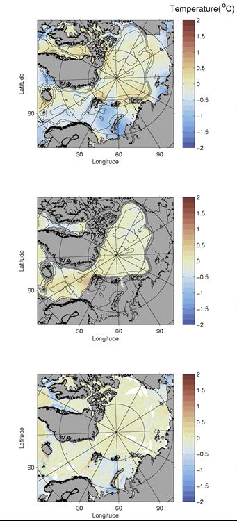
Figure 1: Change in temperature (°C) calculated as differences between the average over 2005-2012 and average over 1995-2004 from surface (top), at 500 m (middle) and bottom (lower). Some artificial land occurs for bottom estimates due to interpolation challenges.
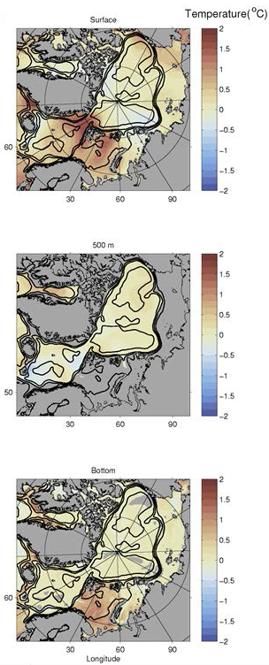
Figure 2: Change in temperature (°C) calculated as differences between the average over 2005-2012 and average over 1995-2004 (left panels) and 1955-1965 (right panels) from surface (top panels), at 500 m (middle panels) and bottom (lower panels). Some artificial land occurs for bottom estimates due to interpolation challenges.
NOAA also has an option to create images using the COBE-SST2 data, a monthly or long term mean of sea surface temperatures, with data between 1850 and 2016. GrADS Images can be created using the website, but the level of detail is quite low and the amount of data is so large, only limited time frames can be selected. For example, a 10-year period is already too long. A one year period gives the image as presented in Figure 3.
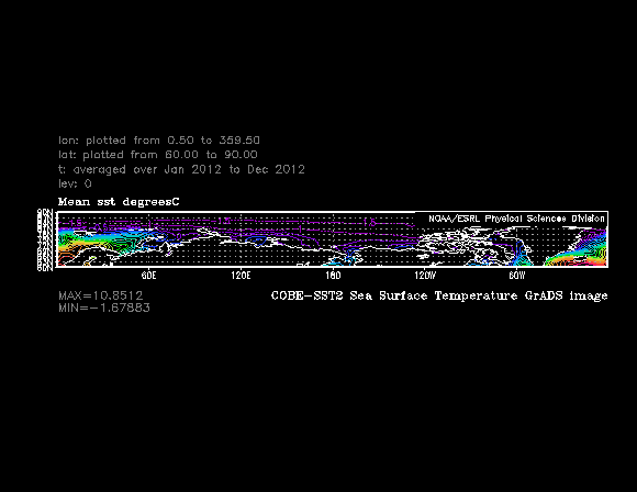
Figure 3: Sea Surface temperatures according to COBE-SST2
The Extended Reconstructed Sea Surface Temperature (ERSST) v4 dataset was used for the Temperature time-series sub-challenge, but monthly gridded data were also available in ASCII and NetCDF format. To create an online viewer of this data, would require programming effort to convert the data into workable formats before publishing it. The UK Met Office offers a similar dataset.
Data use, availability and gaps
Because of the wide breadth of the research question, several decisions were made to make the sub-challenge manageable. . It was decided to work with climatologies instead of single point data. This decision was made to limit the amount of work to put into the product. The climatologies offered an already averaged overview of time and space. Unfortunately, the level of detail of climatologies and precision of the end product is lower compared to using individual point measurements. However, this also solved the problem of data gaps; as the data is averaged to create the continuous data sets. When using individual data points a lot of spatial and temporal gaps will be visible.
Conclusion and lessons learned
In conclusion, there was enough data available to complete this sub-challenge. A lot of data was available, both in climatology form as in individual form. The real task in this challenge was to find the exact dataset required to answer specific questions. In the case of 10 and 50 year time spans, data needed to be available both temporally and spatially, which was not always the case. During the past 10 and 50 years, monitoring strategies have changed and priorities have shifted back and forth, creating gaps in knowledge and data. These gaps cannot be filled as we cannot go back in time to add monitoring points or change the monitoring strategy. However, we can learn from the gathered data (and the missing data) in setting up new monitoring strategies. Sea temperature is directly related to climate change and keeping track of water temperature, especially in the Arctic area, can be very useful in monitoring and evaluating the effects of climate change.
Recommendations
For the future, long term reliable datasets are needed to assess and predict changes in the Arctic system. It is recommended to link physical to biological parameters to understand the entire system and its ongoing change. For water temperature, the requirement of specific data needs to be clearly defined. The use of averaged data needs to be evaluated, in comparison with point data and internal energy of the water.
References:
- Boyer, P., J.I. Antonove, O.K. Baranova, H.E. Garcia, D.R. Johnson, T.P. Locarinini, A.V. Mishonov, D.K. O'Brien, D. Seidov, I. Smolyar, M.M. Zweng (2009). World Ocean Database, 2009. U.S. Government Printing Office, National Oceanic and Atmospheric Administration. ftp://ftp.nodc.noaa.gov/pub/WOD/DOC/wod09_intro.pdf
- Folland, C. K. and D. E. Parker, 1995: Correction of instrumental biases in historical sea surface temperature data. Q. J. R. Meteorol. Soc., 121, 319-367.
- Hirahara, S., Ishii, M., and Y. Fukuda, 2014: Centennial-scale sea surface temperature analysis and its uncertainty. J of Climate, 27, 57-75. http://journals.ametsoc.org/doi/pdf/10.1175/JCLI-D-12-00837.1
- Huang, B., V.F. Banzon, E. Freeman, J. Lawrimore, W. Liu, T.C. Peterson, T.M. Smith, P.W. Thorne, S.D. Woodruff, and H.-M. Zhang, 2014: Extended Reconstructed Sea Surface Temperature version 4 (ERSST.v4): Part I. Upgrades and intercomparisons. Journal of Climate, 28, 911–930, doi:10.1175/JCLI-D-14-00006.1 (link is external). http://journals.ametsoc.org/doi/pdf/10.1175/JCLI-D-14-00006.1
- Huang, B., P. Thorne, T. Smith, W. Liu, J. Lawrimore, V. Banzon, H. Zhang, T. Peterson, and M. Menne, 2015: Further Exploring and Quantifying Uncertainties for Extended Reconstructed Sea Surface Temperature (ERSST) Version 4 (v4). Journal of Climate, 29, 3119–3142, doi:10.1175/JCLI-D-15-0430.1 (link is external). http://journals.ametsoc.org/doi/pdf/10.1175/JCLI-D-15-0430.1
- Ishii, M., A. Shouji, S. Sugimoto, and T. Matsumoto, 2005: Objective Analyses of Sea-Surface Temperature and Marine Meteorological Variables for the 20th Century using ICOADS and the Kobe Collection. Int. J. Climatol., 25, 865-879. http://onlinelibrary.wiley.com/doi/10.1002/joc.1169/pdf
- Japan Meteorological Agency, 2006: Characteristics of Global Sea Surface Temperature Analysis Data (COBE-SST) for Climate Use. Monthly Report on Climate System Separated Volume, 12, 116pp. http://ds.data.jma.go.jp/tcc/tcc/products/elnino/cobesst_doc.html
- Liu, W., B. Huang, P.W. Thorne, V.F. Banzon, H.-M. Zhang, E. Freeman, J. Lawrimore, T.C. Peterson, T.M. Smith, and S.D. Woodruff, 2014: Extended Reconstructed Sea Surface Temperature version 4 (ERSST.v4): Part II. Parametric and structural uncertainty estimations. Journal of Climate, 28, 931–951, doi:10.1175/JCLI-D-14-00007.1 (link is external). http://journals.ametsoc.org/doi/pdf/10.1175/JCLI-D-14-00007.1
- Locarnini, R. A., A. V. Mishonov, J. I. Antonov, T. P. Boyer, H. E. Garcia, O. K. Baranova, M. M. Zweng, and D. R. Johnson, 2010. World Ocean Atlas 2009, Volume 1: Temperature. S. Levitus, Ed., NOAA Atlas NESDIS 68, U.S. Government Printing Office, Washington, D.C., 184 pp. ftp://ftp.nodc.noaa.gov/pub/WOA09/DOC/woa09_vol1_text.pdf
- Seidov, D., J. I. Antonov, K. M. Arzayus, O. K. Baranova, M. Biddle, T. P. Boyer, D. R. Johnson, A. V. Mishonov, C. Paver and M. M. Zweng (2015). "Oceanography north of 60°N from World Ocean Database." Progress in Oceanography 132: 153-173.
- COBE2 files and a README (grib format).
The COBE monitoring dataset is here: Japanese Oceanographic Data Center http://ds.data.jma.go.jp/tcc/tcc/products/elnino/cobesst/cobe-sst.html - https://www.esrl.noaa.gov/psd/data/gridded/data.cobe2.html
- http://www.nodc.noaa.gov/OC5/regional_climate/arctic/
- https://www1.ncdc.noaa.gov/pub/data/cmb/ersst/v4/ascii/
- http://www.metoffice.gov.uk/hadobs/hadisst/data/download.html
- http://www.metoffice.gov.uk/hadobs/hadisst/index.html
Time series of average annual temperature at sea surface and bottom
Sub-challenge: Create time series of average annual temperature at sea surface and bottom.
Results
This sub-challenge was interpreted as the average annual temperature of the entire Arctic area, as defined for this project (The Arctic Ocean as defined in the CIA factbook) and can be divided into two scenarios:
- Time series of average annual temperature at sea surface for the entire study area;
- Time series of average annual temperature at sea bottom for the entire study area.
No time span was indicated in the original sub-challenge (only ‘annual average’) and no spatial scale was indicated.
A time series of average annual temperature at sea surface (1) is available free of charge. For an interactive map with data on water temperature see https://emodnet.ec.europa.eu/geoviewer/ and select “water temperature”. Here you can filter for temperature (and also salinity, conductivity etc.) and select individual locations which will open a new window showing the available measured data. This data is presented differently per location, depending on the data available. Figure 1 shows the interactive map with a selected location.
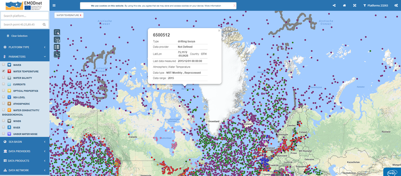
Figure 1: Interactive map with selected location
Figure 2 is a depiction of the sea surface temperature (SST) of the Northern Hemisphere, with the upper limits and lower limits for each year and the calculated sea surface temperature anomalies relative to the mean SST of 1961 until 1990. This data is downloadable free of charge at https://www.metoffice.gov.uk/hadobs/hadsst3/data/download.html. Unfortunately this data shows the mean of the entire Northern Hemisphere, thus showing a very generalised image of the SST, which is not directly applicable to the Arctic Sea. More local data can be easily retrieved using the interactive map mentionedabove. However, the map does not show compared data, like SST anomalies.
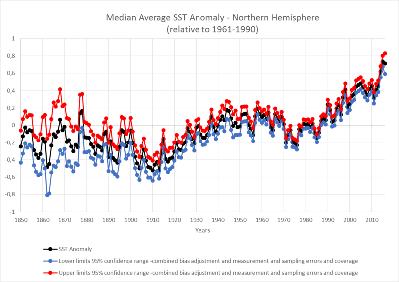
Figure 2: Median average Sea Surface Temperature anomaly for the Northern Hemisphere, datasource: UK Met Office).
The same data trend can be seen on the website of the National Oceanic and Atmospheric Administration (NOAA), showing the SST anomaly of 60 degrees North to 90 degrees North (Arctic circle), depicted in degrees of Kelvin, Figure 3.
https://www.ncdc.noaa.gov/data-access/marineocean-data/extended-reconstructed-sea-surface-temperature-ersst-v4
At the NOAA website you can also find daily updated maps with ocean temperatures: http://www.ospo.noaa.gov/Products/ocean/sst/contour/
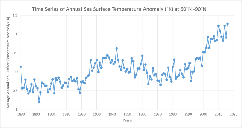
Figure 3: Sea Surface Temperature anomaly, datasource: NOAA.
Timmermans & Proshutinsky (2015) constructed the SST anomalies from three different Arctic seas, Figure 4. This is based on the same data available at the NOAA website. About the dataset:
“Sea surface temperatures are determined using the extended reconstructed sea surface temperature (ERSST) analysis. ERSST uses the most recently available International Comprehensive Ocean-Atmosphere Data Set (ICOADS) and statistical methods that allow stable reconstruction using sparse data. The monthly analysis begins January 1854, but due to very sparse data, no global averages are computed before 1880. With more observations after 1880, the signal is stronger and more consistent over time.” (www.ncdc.noaa.gov)
The graph shows considerable variation between the different seas, indicating that when using the mean SSTs for the entire Arctic, important information might be overlooked.
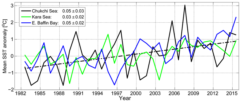
Figure 4: Time series of area-averaged SST anomalies [°C] for August of each year relative to the August mean for the period 1982-2010 for the Chukchi and Kara seas and eastern Baffin Bay. The dash-dotted black line shows the linear SST trend for the Chukchi Sea (the same warming trend as eastern Baffin Bay). Numbers in the legend correspond to linear trends (with 95% confidence intervals) in °C/year (source: Timmermans & Proshutinsky, 2015).
Information about the sea bottom temperature is scarce. Rabe et al. (2015) described the surface and bottom sea temperature from 86 locations which were visited consecutively in the year 2012 (Figure 5). The data can be downloaded free of charge from the Pangea website (www.pangaea.de).
This data treats all locations as 1 sampling site, meaning that local differences are not accounted for.
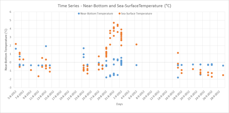
Figure 5: Sea Surface and Bottom Temperature in 2012, datasource: Rabe et al., 2015.
In the period from 2007 until 2014, Russian-German research programs operated a series of year-round oceanographic moorings in the Laptev Sea, which provide a nearly continuous hydrographic record from the central shelf (Janout et al. 2016). This data was analysed by Janout et al. (2016), Figure 6 shows the graph from the paper in which the mid-water and bottom water temperatures are depicted.
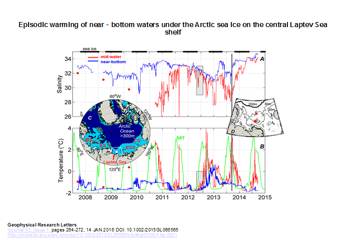
Figure 6: The 2007–2014 mooring record: (a) near-bottom water (blue) and midwater (red) salinity and (b) temperature. The data was smoothed using a 2-day running mean to remove high-frequency variability. Areal-mean SSTs [Reynolds et al., 2002] are included for comparison (green). Red dots in the first half of the record indicate midwater values from CTD profiles. Note that the September 2013 to September 2014 deployment is ~146km north of the previous location; the black dashed line marks the transition time. Black bars at the top of Figure 1a indicate ice cover [Cavalieri et al., 1996]. (c) The white star marks the mooring location. Letters mark adjacent shelf seas: Barents (BS), Kara (KS), East Siberian (ESS), and Chukchi (CS) Seas. Light blue shading indicates regions
Temporal data of SST and bottom sea temperature, can also be found in the sub-challenge: Change in average temperature at surface, 500 metre depth and bottom on a grid over the past 10 years and 50 years. Here data was discussed from the World Oceanic Atlas (WOA), which is available free of charge, concluding that the data requires careful analysis. Therefore, the analysis from a recently published paper (Seidov et al., 2015) was used (available at http://www.nodc.noaa.gov/OC5/regional_climate/arctic/).
Data sets are available from WOA for the periods 1955-64, 1965-74, 1975-84, 1985-94, 1995-2004 and 2005-2012. For this challenge, the most recent data was used to calculate the 10 year change (Figure 1); for the 50 year period they used the difference between 2005-2012 and 1955-1965 (Figure 2).

Figure 1: Change in temperature (°C) calculated as difference between the average over 2005-2012 and average over 1995-2004 from surface (top), at 500 m (middle) and bottom (lower). Some artificial land occurs for bottom estimates due to interpolation challenges.

Data use, availability and gaps
There is sufficient data available on sea surface temperature, but less so for bottom temperature. The available data is mostly point-data from measuring stations. This can be seen in the sub-challenge ‘temperature change on a grid’, different spatial areas can show different changes in temperature. When averaging the entire Arctic area, it would give an inaccurate impression of reality.
All but one dataset can be downloaded free of charge. However, the dataset with the most information regarding sea bottom temperatures is unavailable. The downloadable data sets can be found on the following websites:
- https://emodnet.ec.europa.eu/geoviewer/
(interactive map with point data) - http://www.metoffice.gov.uk/hadobs/hadsst3/data/download.html
(SST anomalies Northern hemisphere) - https://www.ncdc.noaa.gov/data-access/marineocean-data/extended-reconstructed-sea-surface-temperature-ersst-v4
(ERSST data for SST anomalies Arctic and for three arctic seas separately) - http://icoads.noaa.gov/products.html
(ICOAD dataset; basis for the ERSST data) - https://doi.pangaea.de/10.1594/PANGAEA.849735
(2012 cruise by Rabe et al. 2016) - https://www.nodc.noaa.gov/OC5/indprod.html
(WOA dataset)
Conclusion and lessons learned
This sub-challenge was divided into two scenarios:
- Time series of average annual temperature at sea surface for the entire study area;
- Time series of average annual temperature at sea bottom for the entire study area.
For the first scenario the information and data were available. Although a time series, with adjustable time periods, could not be found. Still, the data to construct such time series is present and downloadable free of charge.
For the second scenario there is less information available. Free available information was limited to research over the course of one year (2012) on different locations and comparative data from set time periods. A time series from sea bottom temperature between 2007 until 2014 was found in a research paper. This paper was not available free of charge and there was no option online for retrieving the dataset.
A limitation for both scenarios is that when averaging the temperatures from the entire arctic into one mean temperature important local differences get overlooked.
Recommendations
The interactive map on the Emodnet website is already very informative. But it might hold more potential. The possibility to select multiple locations and compare them in some way could be an upgrade. Especially when available data could be combined and plotted to create comparative time series.
Another recommendation would be to retrieve the dataset from Janout et al. (2016) and make it publicly available, this dataset holds the most comparative data regarding sea bottom temperature and is a necessary addition to the compiled data.
References:
Literature
- AMAP, 2012. Arctic Climate Issues 2011: Changes in Arctic Snow, Water, Ice and Permafrost. SWIPA 2011, Overview report. (https://www.amap.no/documents/doc/arctic-climate-issues-2011-changes-in-arctic-snow-water-ice-and-permafrost/129)
- Janout, M., J. Hölemann, B. Juhls, T. Krumpen, B. Rabe, D. Bauch, C. Wegner, H. Kassens & L. Timokhov, 2016. Episodic warming of near-bottom waters under the Arctic sea ice on the central Laptev Sea shelf. Geophysical Research Letters 43(1): 264-272. (http://onlinelibrary.wiley.com/doi/10.1002/2015GL066565/full)
- NOAA (2015) Arctic Report Card: Update for 2015
- Rabe, Benjamin; Kikuchi, Takashi; Wisotzki, Andreas (2015): Physical oceanography from 86 XCTD stations during POLARSTERN cruise ARK-XXVII/3 (IceArc). doi:10.1594/PANGAEA.849735 https://doi.pangaea.de/10.1594/PANGAEA.849735
- Timmermans, M.L. & a. Proshutinsky, 2015. Sea surface Temperature. In: Arctic Report Card: Update for 2015.
Websites
- http://www.nunatsiaqonline.ca/stories/article/656742015_noaa_arctic_report_card_shows_increased_heat/
- https://www.innovation.ca/sites/default/files/Rome2013/files/SWIPA%20Overview%20Report%202011.pdf
- https://www.ncdc.noaa.gov/data-access/marineocean-data/extended-reconstructed-sea-surface-temperature-ersst-v4
- http://www.nodc.noaa.gov/OC5/regional_climate/arctic/
- https://hypertextbook.com
- http://icoads.noaa.gov/index.shtml
- http://www.cru.uea.ac.uk/
- http://www.metoffice.gov.uk/hadobs/hadsst3/data/download.html
- ftp://ftp.ncdc.noaa.gov/pub/data/noaaglobaltemp/operational/timeseries/
Internal energy (time-series)
Sub-challenge: time-series of average annual internal energy of sea
The internal energy of the sea can mean many things; mechanical motions like waves and currents contain energy (BOEM (Bureau of ocean energy management)); energy created by external forces like wind, tides, freshwater input and atmospheric pressure also add energy to, or deplete the ocean of energy; or thermal energy like geothermal heat or air-sea latent heat (Ferrari, R.; Wunsch, 2008). In physics chemical bonds and potential energy within an object would also be considered part of the internal energy as it is all the energy contained in a system (HyperPhysics). The ocean also has a heat content which tracks warm water flows and is used in the prediction of El Niño and La Niña events (National Oceanic and Atmospheric Administration). If we consider the internal energy of the Arctic sea, the majority of internet search results involve energy derived from mixing and internal waves. However, if we consider the internal energy of sea ice the majority of internet searches result in data on thermal energy.
Even if we consider either wave energy or thermal energy in sea as internal energy, it is still a complex challenge. Thermal dynamics of sea in the arctic area also involve the complex thermal dynamics of sea ice. Thermal energy in sea ice can be caused by shortwave radiating heat, within the sea ice. As this energy warms the ice from the inside, brine pockets can develop. These pockets store latent heat, melting the ice from the inside out. The amount of heat capacity and thermal conductivity following this is dependent on the temperature and salinity of the sea ice (McCaa, 2004). Furthermore, data (GIS) can also be found on wave energy (National Snow and Ice Data Center) but is generally focussed on wave energy at coastlines rather than in the open ocean.
Results:
Data on heat content of the entire ocean is available and is used in the prediction of El Niño and la Niña events (Ocean Climate Laboratory (OCL) of National Oceanographic Data Center (NODC)). Data is however limited to the resolution of the entire ocean or Northern or Southern hemispheres, and lacks the detail of smaller scale, specific areas. It does however have a temporal range from 1955 until 2017.
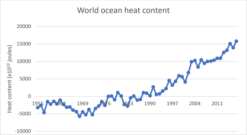
Figure 1 Source: https://www.nodc.noaa.gov/OC5/3M_HEAT_CONTENT/basin_data.html
Data use, availability and gaps
For this challenge there is no definite conclusion on the availability of data. There is no data found when searching keywords such as ‘internal energy’ is used. However internal energy contains all of the energy in a system. Quite often parts of the internal energy like thermal energy or wave energy are documented. Actual data on the entire internal energy means combining all separate elements of internal energy; this is a huge task given data sets are on different temporal and spatial scales.
Conclusion and lessons learned
The question asked in this challenge needs to be reviewed and made explicit. Is it necessary to have specific information on the internal energy of the sea, including mechanical energy, external energy and thermal energy and potential energy? Or is there a need for data on subsets of internal energy like thermal energy or wave energy?
Recommendations
The internal energy of the sea is not a very well-known parameter, even though it has a direct relationship with Climate Change. Monitoring for Internal energy means monitoring for all the component parts of internal energy and it is quite time and cost intensive. For this reason, we do not recommend an extension of the current challenge. Further extension of specific research should always be promoted, especially considering climate change. However, we recommend research on more obvious parameters, like thermal or wave energy.
References:
- BOEM (Bureau of ocean energy management). (n.d.). Ocean Wave Energy. Retrieved March 5, 2018, from https://www.boem.gov/renewable-energy/renewable-energy-program-overview
- Ferrari, R.; Wunsch, C. (2008). Ocean Circulation Kinetic Energy—Reservoirs, Sources and Sinks: Supplementary Material. Annu. Rev. Fluid Mech. Retrieved from https://www.annualreviews.org/article/suppl/10.1146/annurev.fluid.40.111406.102139?file=fl.41.ferrari.pdf
- HyperPhysics. (n.d.). Internal Energy Concepts. Retrieved March 7, 2018, from http://hyperphysics.phy-astr.gsu.edu/hbase/thermo/intengcon.html#c1
- McCaa, J. (n.d.). 6.6 Brine Pockets and Internal Energy of Sea Ice. Retrieved March 5, 2018, from http://www.cesm.ucar.edu/models/atm-cam/docs/description/node38.html
- National Oceanic and Atmospheric Administratio. (n.d.). NOAA Climate.gov - Heat Capacity of Water. Retrieved March 7, 2018, from https://www.climate.gov/taxonomy/term/8390/feed
- National Snow and Ice Data Center. (n.d.). Arctic Coastal Dynamics Database, Version 2. Retrieved March 7, 2018, from http://nsidc.org/data/GGD629
- Ocean Climate Laboratory (OCL) of National Oceanographic Data Center (NODC). (n.d.). Global Ocean Heat Content: Basin time series. Retrieved March 7, 2018, from https://www.nodc.noaa.gov/OC5/3M_HEAT_CONTENT/basin_data.html
Ice cover (grid)
Sub-challenge: Change in average ice cover (kg m2/year) over the past 10 years, past 50 years and past 100 years, shown on a grid.
Results
The task was to find data on changes in average ice cover over past 10 years, past 50 years and past 100 years, and present these on a grid. This means the sub-challenge can be divided into three different scenarios:
- Change in average ice cover (kg m2/year) over the past 10 years shown on a grid for the entire study area;
- Change in average ice cover (kg m2/year) over the past 50 years shown on a grid for the entire study area;
- Change in average ice cover (kg m2/year) over the past 100 years shown on a grid for the entire study area.
To calculate change in ice cover (kg m2/year) estimates of ice thickness and, ideally, ice density are necessary in addition to ice extent and concentration. There are different methods for measuring ice thickness, e.g. in situ from the surface, upward looking sonars (mounted on submarines or moorings), or remote sensing (satellite and airborne LIDAR observations (Light Detection and Ranging – a detection system similar to radar but uses laser generated light). An overview of available data and associated uncertainty are presented in a recent paper by Lindsay and Schweiger (2015). According to Lindsay and Schweiger; "Historically, a great number of ice thickness measurements have been made at specific locations using drill holes or ground based electromagnetic methods; however, these point measurements are difficult to translate into area-averaged mean ice thickness because of the highly heterogeneous nature of the ice pack." For this reason, no historical observational data could be used to map changes in ice thickness over the last 50 and 100 years.
There are several data sets available from the U.S. National Snow and Ice Data Center (NSIDC) at the University of Colorado. The most useful in this context is the Unified Sea Ice Thickness Climate Data Record Collection Spanning 1947-2012 (Lindsay 2013). This is the dataset used and described in Lindsay and Schweiger (2015). Starting from 2010 estimates of ice thickness are available from the European Space Agency’s CryoSat-2 satellite. ESA Data is available from Centre for Polar Observation and Modelling at the University College London (cpom.ucl.ac.uk) (Laxon, Giles et al. 2013). However, there was no dataset available on change in average ice cover as requested, and estimates must therefore were made from available data on ice extent and ice thickness (assuming a constant density of sea ice). Obtaining good measurements of average ice thickness over the last decade was challenging because of the sparsity of data in space and time. For the past 50 and 100 years it was not possible, as discussed above. An alternative method is using model data. Data from the University of Washington’s Pan-Arctic Ice Ocean Modeling and Assimilation System (PIOMAS) is available (Zhang et al. 2013). A description and evaluation of the performance of this system to simulate ice thickness is found in Schweiger, Lindsay et al. (2011). We downloaded PIOMAS area and ice thickness data. By assuming a constant ice density of 930 kg/m3 we calculated the trend in average ice cover (kg m2/year) over the last decade (2006-2015) (Figure 1).
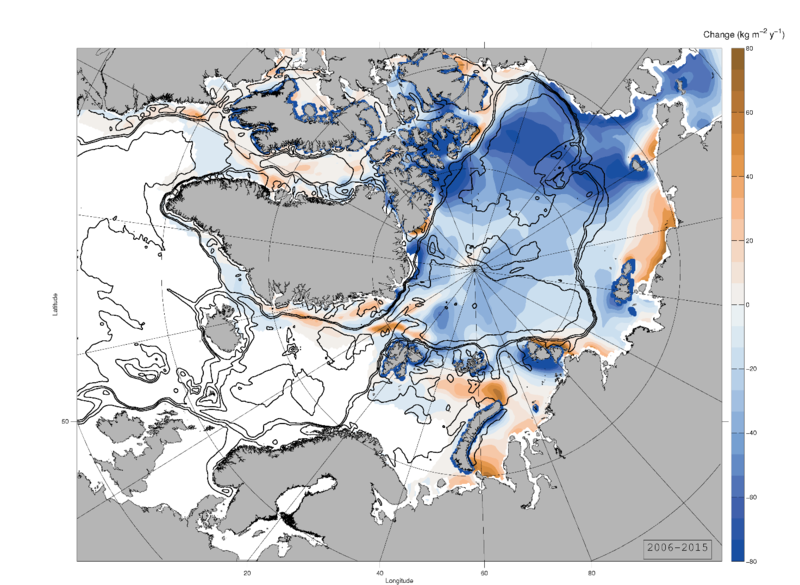
Figure 1: Trend in average ice cover (kg m-2 y-1) over the last decade (2006-2015).
Data use, availability and gaps
There was not enough data available to complete this sub-challenge . We were unable to locate reliable data specific to average ice cover in kg m2 /year for the past 50 or 100 years. A ‘grid’ was added to the maps for optimal viewing. Data are from U.S. NOAA and from European Space Agency and University of Washington, U.S.A.
Conclusion and lessons learned
In all the data sets, the decline in the extent of solid ice is notable, though more so in the Atlantic sector than in the Bering Sea sector. However, as sea ice thickness is different from extent, different research techniques are necessary and these produce different data. Lessons learned during this sub-challenge:
- Data on sea-ice thickness (especially in kg m2 /year) was not readily available as it was a hard to measure.
- More data on ice thickness is becoming available relatively recently with new measuring techniques and the use of models.
Recommendations
Sea-ice thickness is an important parameter for climate change research and we recommend a yearly monitoring programme.
References:
- Laxon, S. W., K. A. Giles, A. L. Ridout, D. J. Wingham, R. Willatt, R. Cullen, R. Kwok, A. Schweiger, J. Zhang, C. Haas, S. Hendricks, R. Krishfield, N. Kurtz, S. Farrell and M. Davidson (2013). "CryoSat-2 estimates of Arctic sea ice thickness and volume." Geophysical Research Letters 40(4): 732-737.
- Lindsay, R. (2013). Unified Sea Ice Thickness Climate Data Record Collection Spanning 1947-2012, version 1. Boulder, Colorado, USA, National Oceanic and Atmospheric Administration, National Snow and Ice Data Center.
- Lindsay, R. and A. Schweiger (2015). "Arctic sea ice thickness loss determined using subsurface, aircraft, and satellite observations." The Cryosphere 9(1): 269-283.
- Zhang, Jinlun and D.A. Rothrock: Modeling global sea ice with a thickness and enthalpy distribution model in generalized curvilinear coordinates, Mon. Wea. Rev. 131(5), 681-697, 2003. http://psc.apl.washington.edu/zhang/IDAO/data_piomas.html
- http://www.cpom.ucl.ac.uk/csopr/seaice.html
Ice cover (map)
Sub-challenge: Average extent of ice coverage over past 5 years, past 10 years, past 50 years, past 100 years, plotted on maps.
Results
This challenge was split into four different scenarios:
The data set we found that contains the oldest historical data is from the NOAA / National Environmental Satellite, Data and Information Service (NESDIS) / National Snow and Ice Data Center (NSIDC) at the University of Colorado. The Gridded Monthly Sea Ice Extent and Concentration, 1850 Onwards, version 1. These data were recently released by Walsh, Chapman et al. (2016). Sea ice concentration is a proxy for ice coverage, e.g. 15%-20% ice concentration is considered a reasonable definition of "covered", and, if combined with an estimate of ice density and thickness information, it is possible to estimate coverage (kg m2/year). Ice coverage is an important consideration for determining when an ice class vessel is required. Error in ice concentration estimates is generally on the order of 5%, but can be greater (nsidc.org). The older data are monthly gridded data based on ship observations, naval oceanographer records, and analysis by different national ice services (see Table 1). Satellite passive microwave data began to collect full Arctic data in 1979. Full data sets were first published in 1991 (with historical data back to the 1990s). These new data are intended to be used as boundary conditions for model applications such as reanalyses (e.g. model runs to simulate historical conditions or climatologies). Although these data show the decrease in area, they do not show how significantly sea ice thickness has declined over the last six decades. Kwok and Rothrock (2009) use declassified submarine data to show that the average sea ice thickness at the end of the melt season has decreased by 1.6 m (53%) over 40 years in the area of interest, with negative trends in all regions.
Table 1: Sea Ice Data Sources used by NSIDC. Table from page 5 of Walsh et al (2016). Note that numbers 6,7,14,15 and 19 are not used as they are placeholders for the processing software.
| Value | Data Source |
| 1 | DMI yearbook narrative |
| 2 | JMA charts |
| 3 | NAVO yearbooks |
| 4 | Kelly ice extent grids |
| 5 | Walsh and Johnson |
| 8 | Satellite passive microwave |
| 9 | ACSYS |
| 10 | AARI |
| 11 | Hill |
| 12 | Dehn |
| 13 | Danish Meteorological Institute |
| 16 | Whaling log books open water |
| 17 | Whaling log books partial sea ice |
| 18 | Whaling log books sea ice covered |
| 20 | Analog filling of spatial gaps |
| 21 | Analog filling of temporal gap. |
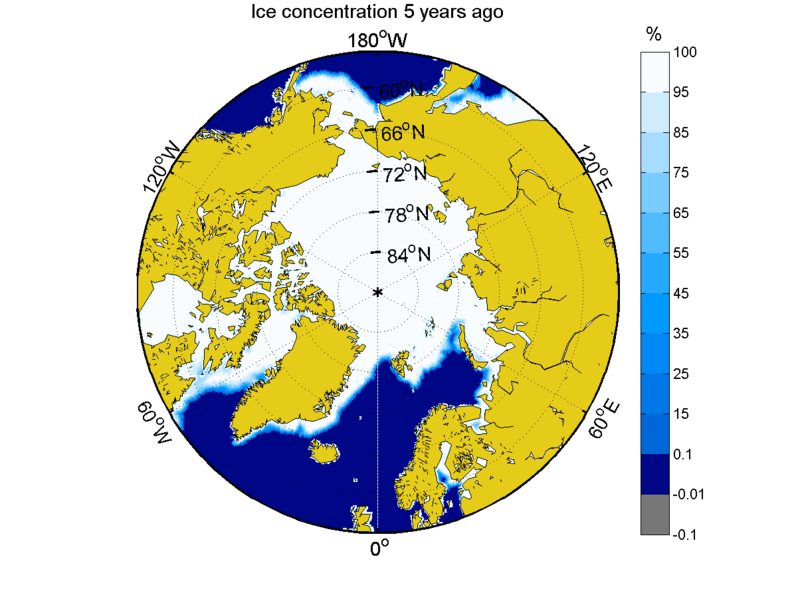
Figure 5: Map of Sea Ice Concentration 5 years ago (from 2016). Data from Walsh, Chapman et al. (2016). Consider 15% concentration as the lower boundary for ice coverage. March is shown, as that is the month of maximum sea ice extent.

Figure 6: Map of Sea Ice Concentration 10 years ago (from 2016). Data from Walsh, Chapman et al. (2016). Consider 15% concentration as the lower boundary for ice coverage. March is shown, as that is the month of maximum sea ice extent.
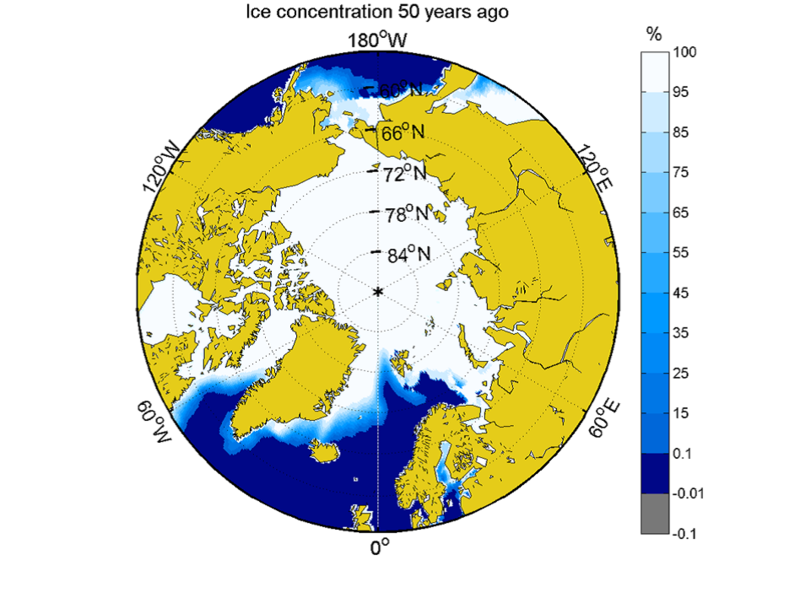
Figure 7: Map of Sea Ice Concentration 50 years ago (from 2016). Data from Walsh, Chapman et al. (2016). Consider 15% concentration as the lower boundary for ice coverage. March is shown, as that is the month of maximum sea ice extent.
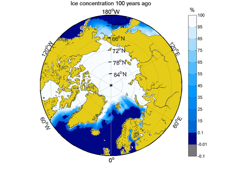
Figure 8: Map of Sea Ice Concentration 100 years ago (from 2016). Data from Walsh, Chapman et al. (2016). Consider 15% concentration as the lower boundary for ice coverage. March is shown, as that is the month of maximum sea ice extent.
Data use, availability and gaps
Enough data was available to complete this sub-challenge. We used the data from U.S. NOAA. It was chosen to add a ‘grid’ to the maps for optimal viewing. However, one must keep in mind that historical Arctic data from more than a few decades ago is very different from modern data due to the changes in sampling methods (e.g. invention of the CTD, and initiation of polar orbiting satellites) and sample locations from individual expeditions to full polar coverage. Archival data is increasingly being merged into digital forms so that historical conditions can be reconstructed. Older data are becoming more available as more reanalysis data sets become available, e.g. Walsh et al (2016) we recently published. Quantities such as "ice concentration" (numerical model friendly), rather than "ice coverage" (shipping terminology), are available due to their use in climate scale numerical simulations, so the key records related to these parameters are the first to be put into synthesized digital forms. As more historical data become available in digital forms, we expect reanalyses of more types of ice information to become available.
Conclusion and lessons learned
A clear decrease in sea-ice extent was seen.
Recommendations
It is very important to keep track of Sea-ice extent on a scientific level because it is directly related to climate change. Many research projects on sea-ice are already in place, however it is useful to combine and join efforts and results to create an overview for the entire Arctic area.
References:
- Average extent of ice coverage over the past 5 years of the entire study area plotted on a map;
- Average extent of ice coverage over the past 10 years of the entire study area plotted on a map;
- Average extent of ice coverage over the past 50 years of the entire study area plotted on a map;
- Average extent of ice coverage over the past 100 years of the entire study area plotted on a map.
- More information on sea-ice extent is available than on sea-ice thickness.
- Measuring techniques have changed significantly over the past 100 years so data is not always comparable.
- Kwok, R., D.A. Rothrock (2009) "Decline in Arctic sea ice thickness from submarine and ICESat records: 1958-2008" Geophysical Research Letters 36 L15501, doi:10.1029/2009GL039035.
- Walsh, J. E., W. L. Chapman and F. Fetterer (2016). Gridded Monthly Sea Ice Extent and Concentration, 1850 Onward, Version 1. https://nsidc.org/data/g10010.
Ice cover (time series)
Sub-challenge: Total ice cover in sea (kg) over past 100 years plotted as time series
While sea ice cover is generally measured in kg and the data then calculated as ‘ice mass’ (kg/m^2), the majority of data collected does not cover actual sea ice mass. Sea ice mass balance is the gain and loss of sea-ice from the Arctic. This is most often calculated by using extent and thickness data alongside data on ice surface and bottom melt, sea level pressure, heat fluxes and surface air temperature and says more about the thermodynamics of sea ice then about the total amount of cover. So although data on sea-ice mass balance is available it mostly shows the growth and melting of ice in centimetres (Cold regions research and engineering lab, 2018).
When looking at Sea Ice cover the majority of the data available is focussed on sea ice extent or sea ice thickness. As weight not only depends on area size and thickness, but also on the density and age of the ice or snow (Richter-Menge et al., 2006), it is difficult to determine the mass weight. Nevertheless, to create a time-series on the sea-ice cover it was most practical to focus on using sea-ice extent and thickness as parameters instead of mass. These parameters are widely available for download from various websites.
Arctic researchers are aware of the need for data sharing. Multiple collaborations like APECS, the Association of Polar Early Career Scientists, are investing in data management and making data from the polar regions publicly available. Through their website multiple other databases were accessed, including https://www.polardata.ca/pdcsearch/. This site presents various studies and data sets from research performed in the Arctic region, however not all are publicly available and none cover the entire arctic or a time span of 100 years.
Results
Sea Ice Extent
Data on extent are widely available through websites like National snow and ice data centre (nsidc.org). All data are available free of charge, but for most data a (cost free) registration is required as websites often use FTP directories to exchange data. Most of the data available began from 1979, the beginning of satellite data (Kattsov et al., 2010).
Each subset of data has its own page describing not only the data in the files, but also the way these were obtained and filed. Explanations of file names, parameters and variables are present on this page. The nsidc website can be searched through this page (http://nsidc.org/data/search/).
For Sea ice extent specifically one of the databases on the northern hemisphere can be downloaded through an FTP directory. An FTP is a File transport protocol, which enables data transport between a computer and a server. Using at least windows 10, connection to the FTP directory can be made by adding a new network location in the file directory.
The FTP used contains data NOAA data on sea ice extent (NSIDC; NOAA, 2018) in the Northern and southern hemisphere. Using Northern hemisphere data, the following timeline of sea ice extent could be produced. This data is generated by Fetterer, F., K. Knowles, W. Meier, M. Savoie, 2017
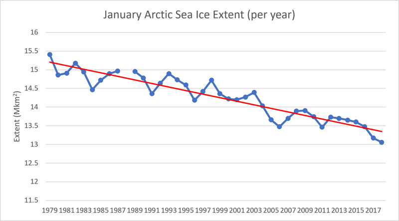
Figure 1: Sea Ice extent in the Northern Hemisphere in January, from 1979 to 2016, in million square km.
Data for figure 2 was downloaded from the Blue ice website. This data opened in a webpage, which could be converted to a text-file and imported into Excel. The temporal resolution is 1979-2007 and contains data on nine different sample sites throughout the Arctic. These nine sites are combined by the data-collectors into a total amount of sea ice extent for the entire Arctic. The data was used for multiple papers on sea ice cover (Cavalieri, D. J., C. L. Parkinson, P. Gloersen, J. C. Comiso, 1999; Cavalieri, D. J., P. Gloersen, C. L. Parkinson, J. C. Comiso, 1997; Gloersen, P., C. L. Parkinson, D. J. Cavalieri, J. C. Comiso, 1999; Gloersen, P., W. J. Campbell, D. J. Cavalieri, J. C. Comiso, C. L. Parkinson, 1992; Parkinson, C. L., D. J. Cavalieri, P. Gloersen, H. J. Zwally, 1999; Parkinson, C. L., 2002; ).
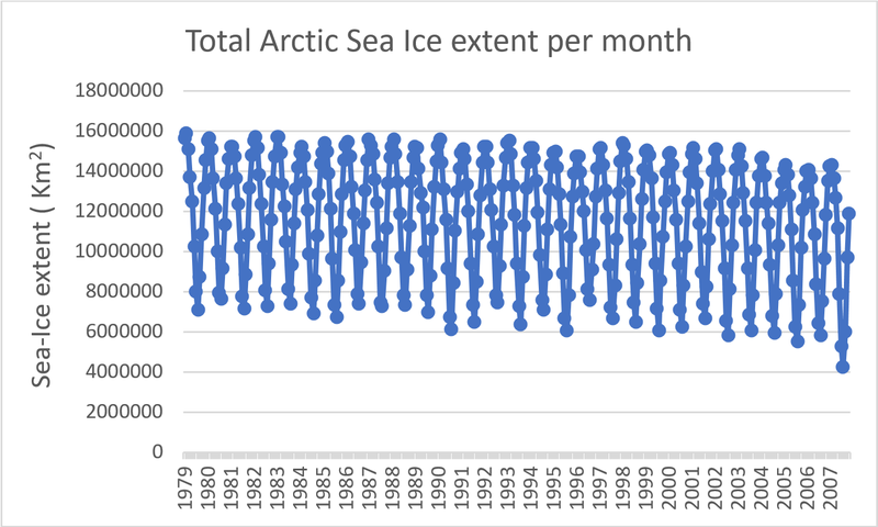
Figure 2. Monthly extent of sea ice in the arctic. From source: https://blueice.gsfc.nasa.gov/seaice_datasets.html (Extent Monthly)
Sea-Ice Thickness
The dataset with the biggest temporal resolution on sea ice thickness is available from Nsidc, this data is gathered using upward looking sonar and has a temporal range from 1960 until 2005. It includes data from the Royal Navy and U.S. military submarines. Although governmental submarines, the data collected is not classified and is therefore available with date and location (National snow and ice data center).
This data can be downloaded through an FTP directory and is provided in .tgz files, which can be opened using software like Winzip.
The data however is organised per year, with each year having different submarine tracks. This means that although the majority of the Arctic is covered it is difficult to make an accurate time series as no two measurement points are the same. Points can be divided into areas which would allow year by year comparison, but this is a time-consuming exercise. This data has been used to present the decline of sea ice thickness over time (Kwok & Rothrock, 2009; Rothrock, Yu, & Maykut, 1999).
Zwally, Yi, Kwok, & Zhao (2008) also provide data on sea ice thickness through the Nsidc website (requires a free Earthdata account). However, the data is logged in a way that makes it very time consuming to use and ranges only five years, from 2003 to 2008. The data in this database is logged in irregular time periods, and within every time period data is logged to a specific date. On each date a sample run was done using boats. However, these runs do not generate the same sample points for each run. This means that although data is freely available it is inconsistent and requires much manual processing.
Sturm (2009) provides data on sea ice thickness, but only in a two week time period on a single location. Spatially this data only provides insight into the Barrow, Alaska area.
Data on Sea ice thickness is also available via the NSF Arctic Data Centre (Hajo Eicken, Stefan Hendricks, Mette Kaufman, 2009). The temporal coverage is only single flights, done between October 2010 and March 2011. Flights only occur in one location north-east of Barrow Point, Alaska.
Data use, availability and gaps
Major gaps in this challenge included information on ice cover mass; nodata on sea-ice cover mass in kg/m3 was found during this study.
There was a multitude of data found on sea ice extent and thickness. Some data was easy to download and use. Other data, like that from Zwally et al., (2008) needed to be integrated into usable spreadsheets, which was time-consuming. Making graphs from the available data can also be very time consuming due to the way data is stored. Most data sets are categorised in some way, and while there may be up to 40 years of data, the data logging locations vary. Quite often data is logged per month or year, this means that creating a timeline first starts with integrating all those measured months (or years) into one spreadsheet. Various data sets also log data categorised by location. This seems logical, but also required manual combining of data sets to gain insight in the entire Arctic.
The availability of long-term data sets is also a major limitation in this challenge, with the earliest datasets starting in the 1960s.
On the other hand, thickness is measured in meters or centimetres for all data sets, and extent is measured in square kilometers. Data found was presented in Excel, txt, of CSV files, all of which can be easily adjusted for use in Excel.
Conclusion and lessons learned
In conclusion it can be said no data was available on sea ice mass. However, time series can be made using sea ice extent and sea ice thickness. Most of the data sets found have a starting point in the 1960s, when sonar became available, or 1978 when satellites became available. It is near impossible to create a time-series spanning 100 years.
A lot of data concerning sea ice extent is freely available and is regularly updated. Furthermore, scientists are increasingly seeing the need to publicly share data. Getting a total overview of data available on sea ice extent throughout the Arctic requires combining data sets. Only then will true gaps in knowledge become obvious. Keeping track of sea ice extent will eventually lead to a 100 year time series.
Sea ice thickness was a different matter, although data is available, none of it is directly usable. All data needs to be combined, converted or processed before time-series can be made. However, many papers have used time-series created using the available data, suggesting that differently organised data sets do exist.
Recommendations
It is recommended to rephrase the challenge as there is the question of sea ice cover in kg/m3. Is it necessary to have a time-line of sea ice in kg over time? Or would timelines including sea ice extent (km²) or thickness (m) also be sufficient? If sea ice extent and sea ice thickness are desired there is a wide range of research being done and data available.
It is recommended to think about the way data is going to be logged, depending on the nature of the data and its use (images or time series). Consider logging data into one spreadsheet or multiple smaller files. Depending on the question at hand contact with scientists throughout the Arctic region and possibly creating a primary database might be enough to gain full insight into the sea ice extent. No need is seen to generate new research as so much is already being done at this moment. Bringing researchers and their data together however might bring new insights to light.
References:
- Cavalieri, D. J., C. L. Parkinson, P. Gloersen, J. C. Comiso, and H. J. Z. (1999). Deriving Long-Term Time Series of Sea Ice Cover from Satellite Passive-Microwave Multisensor Data Sets. Journal of Geophysical Research, 104, 15,803-15,814.
- Cavalieri, D. J., P. Gloersen, C. L. Parkinson, J. C. Comiso, and H. J. Z. (1997). Observed Changes, Hemispheric Asymmetry in Global Sea Ice. Science (New York, N.Y.), 272, 1104–1106.
- Cold regions research and engineering lab. (2018). Mass balance.
- Fetterer, F., K. Knowles, W. Meier, M. Savoie, and A. K. W. (2017). Sea Ice Index, Version 3. [Subset Extent Northern Hemisphere]. https://doi.org/https://doi.org/10.7265/N5K072F8
- Gloersen, P., C. L. Parkinson, D. J. Cavalieri, J. C. Comiso, and H. J. Z. (1999). Spatial Distribution of Trends and Seasonality in the Hemispheric Sea Ice Covers 1978-1996. Journal of Geophysical Research, 104, 20,827-20,836.
- Gloersen, P., W. J. Campbell, D. J. Cavalieri, J. C. Comiso, C. L. Parkinson, H. J. Z. (1992). Arctic and Antarctic Sea Ice, 1978-1987: Satellite Passive Microwave Observations and Analysis. National Aeronautics and Space Administration, 511, 290.
- Hajo Eicken, Stefan Hendricks, Mette Kaufman, and A. M. (2009). NSF Arctic Data Center. Retrieved February 28, 2018, from https://arcticdata.io/catalog/
- Kattsov, V. M., Ryabinin, V. E., Overland, J. E., Serreze, M. C., Visbeck, M., Walsh, J. E., … Zhang, X. (2010). Arctic sea-ice change: a grand challenge of climate science. Journal of Glaciology, 56(200), 1115–1121. https://doi.org/10.3189/002214311796406176
- Kwok, R., & Rothrock, D. A. (2009). Decline in Arctic sea ice thickness from submarine and ICESat records: 1958-2008. Geophysical Research Letters, 36(15), n/a-n/a. https://doi.org/10.1029/2009GL039035
- National snow and ice data center. (n.d.). Submarine Upward Looking Sonar Ice Draft Profile Data and Statistics, Version 1. Retrieved February 28, 2018, from https://doi.org/10.7265/N54Q7RWK
- NSIDC; NOAA. (n.d.). Sea ice Index. Retrieved from http://nsidc.org/data/G02135
- Parkinson, C. L., D. J. Cavalieri, P. Gloersen, H. J. Zwally, and J. C. C. (1999). Variability of the Arctic Sea Ice Cover 1978-1996. Journal of Geophysical Research, 104, 20,837-20,856.
- Parkinson, C. L., and D. J. C. (2002). A 21-year record of Arctic sea ice extents and their regional, seasonal, and monthly variability and trends. Annals of Glaciology.
- Richter-Menge, J. A., Perovich, D. K., Elder, B. C., Claffey, K., Rigor, I., & Ortmeyer, M. (2006). Ice mass-balance buoys: a tool for measuring and attributing changes in the thickness of the Arctic sea-ice cover. Annals of Glaciology, 44, 205–210. https://doi.org/10.3189/172756406781811727
- Rothrock, D. A., Yu, Y., & Maykut, G. A. (1999). Thinning of the Arctic sea-ice cover. Geophysical Research Letters, 26(23), 3469–3472. https://doi.org/10.1029/1999GL010863
- Sturm, M. and J. S. (2009). AMSRIce03 Sea Ice Thickness Data, Version 1 | National Snow and Ice Data Center. Retrieved February 28, 2018, from http://nsidc.org/data/NSIDC-0426/versions/1
- Zwally, H. J., J. C. Comiso, C. L. Parkinson, D. J. Cavalieri, and P. G. (2002). Variability of Antarctic Sea 1979-1998. Journal of Geophysical Research.
- Zwally, H. J., Yi, D., Kwok, R., & Zhao, Y. (2008). ICESat measurements of sea ice freeboard and estimates of sea ice thickness in the Weddell Sea. Journal of Geophysical Research, 113(C2), C02S15. https://doi.org/10.1029/2007JC004284
Mass of ice lost (or gained) from Greenland expressed as time series
Sub-challenge: The mass of ice lost from Greenland expressed as time series
Results
The impacts of climate change are especially obvious at the ice sheet of Greenland. The ice sheet encompasses a relatively low latitude and has warm-in-summer regions which have warmed by 2°C since the early 1990’s (Hanna et al., 2008). These regions are predicted to further warm between 2 and 12°C during the present century (Gregory, Huybrechts, & Raper, 2004). The Greenland ice sheet has been identified as one of the most sensitive “tipping elements” of global climate change, meaning that once the ice has melted, the decrease in temperature for returning to its previous state would be greater than the increase which caused the melt (Lenton et al., 2008). Over the last 30–50 years the ice sheet has undergone significant increases in its surface melt area and (modelled) runoff, as well as enhanced mass turnover (Hanna et al., 2011).
The Greenland ice sheet holds a massive amount of water and would be responsible for the equivalent of 6–7 m of contemporary sea level rise if it were to melt completely (Cuffey & Marshall, 2000). The estimation of change in total mass balance of the Greenland ice sheet is intricately related to competing changes in mass outflux and influx: while melt and runoff have increased in the past several decades, snow accumulation has also increased (Hanna et al., 2008). Adding to the complexity are anomalous events, detected in long term data sets from satellites, in snow accumulation and snowmelt (Nghiem et al., 2012)
Finding data regarding the changes in mass of the Greenland ice sheet expressed as a time series could provide the necessary information for understanding these changes.
GRACE satellites
The Gravity Recovery And Climate Experiment (GRACE) is a joint NASA-DLR satellite mission. The GRACE twin satellites are orbiting Earth at approximately 500 km and were launched in March 2002. The two satellites are separated by approximately 200 km in space and the relative distance between the two is measured very accurately. This information is used to derive monthly, global models of the Earth’s gravitational field (Barletta, Sørensen, & Forsberg, 2013).
On the website http://polarportal.dk/en/home/ the Danish Arctic Research Institution presents updated knowledge on the condition of two major components of the Arctic: The Greenland ice sheet and the sea ice. Among the information available is an interactive map with an accompaying graph showing the change in ice mass relative to June 2006, Figure 1 and Figure 2. Source: http://polarportal.dk/en/groenlands-indlandsis/nbsp/total-masseaendring/.
The webpage illustrates how the ice sheet gains mass through snowfall accumulating on the surface and how it shrinks through melting from the surface and discharge of icebergs from glaciers that end up in the sea.
The map depicted in figure 1 and 2 illustrates the latest GRACE satellite-derived mass changes.
The depicted graphs in figure 1 and 2 show the change in the total mass balance month by month, measured in gigatonnes (1 Gt is 1 billion tonnes or 1 km3 of water). The left axis on the graph shows how this ice mass loss corresponds to sea level rise contribution. 100 Gt corresponds to 0.28 mm global sea level. All mass changes in the image are relative to June 2006. Since the measurements began in 2002, the smallest April-to-April mass loss was 29 Gt during 2013-2014 and the largest was 562 Gt during 2012-2013.
The figures 1 and 2 are based on the monthly measurements of changes in gravity. Scientists at DTU Space have contributed to developing the methods used to derive ice mass changes from the gravity changes. The raw GRACE satellite data is carefully processed and validated before it is released to the user, and the product presented here might be delayed by 2-3 months. See Barletta et al. 2013, which is downloadable free of charge.
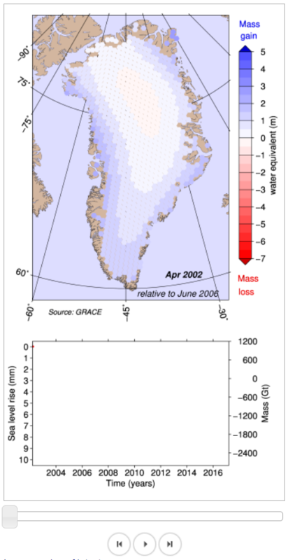
Figure 1: Greenland ice sheet mass gain/loss on April 2002 relative to June 2006 (polarportal.dk)
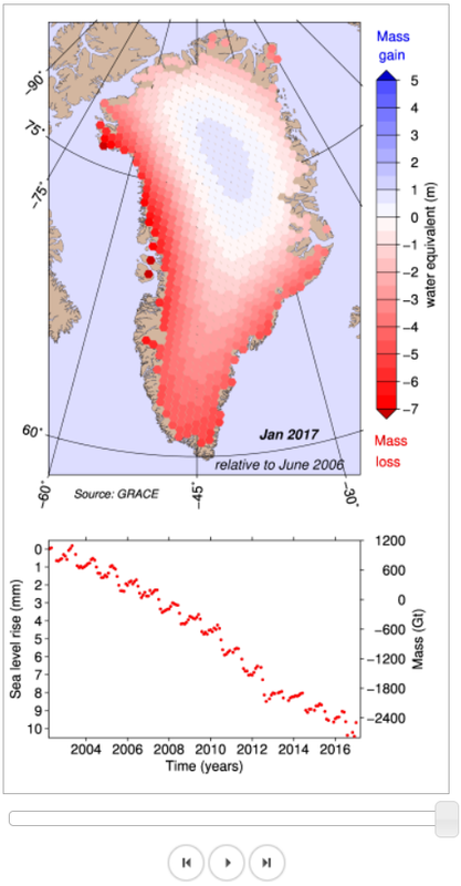
Figure 2: Greenland ice sheet mass gain/loss on January 2016 relative to June 2006 (polarportal.dk)
The GRACE satellite data was also used to create a time series from April 2002 until April 2015, quantifying mass change relative to the first measurement in April 2002, Figure 3 (Tedesco et al., 2015).
An analysis of the mass change data was performed, and this led to several conclusions:
- The melt area in 2015 exceeded more than half of the ice sheet on July 4th for the first time since the exceptional melt events of July 2012, and was above the 1981-2010 average on 54.3% of days (50 of 92 days).
- The length of the melt season was as much as 30-40 days longer than average in the western, north-western and north-eastern regions, but close to and below average elsewhere on the ice sheet.
- Average summer albedo, which is a measure of reflectance, in 2015 was below the 2000-2009 average over the northwest, and above the average over the southwest portion of the Greenland ice sheet. In July, albedo averaged over the entire ice sheet was lower than in 2013 and 2014, but higher than the lowest value on record observed in 2012.
- Ice mass loss of 186 Gt over the entire ice sheet between April 2014 and April 2015 was 22% below the average mass loss of 238 Gt for the 2002- 2015 period, but was 6.4 times higher than the 29 Gt loss of the preceding 2013-2014 season.
- The net area loss from marine-terminating glaciers during 2014-2015 was 16.5 km2. This was the lowest annual net area loss of the period of observations (1999-2015) and 7.7 times lower than the annual average area change trend of -127 km2.
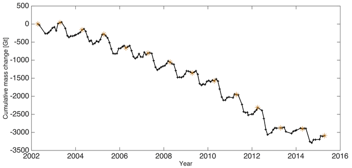
Figure 3: Cumulative change in the total mass (in Gigatonnes, Gt) of the Greenland Ice Sheet between April 2002 and April 2015 estimated from GRACE measurements. Each symbol is an individual month and the orange asterisks denote April values for reference (Tedesco et al., 2015).
Laser altimetry
A study by Zwally et al., 2003, derives mass changes of the Greenland ice sheet for 2003–07 from ICES at laser altimetry and compares them with results for 1992–2002 from ERS radar and airborne laser altimetry. The data is a comparison between two averaged points instead of an entire time series, nevertheless it is very useful and informative.
The data in this paper shows that the Greenland ice sheet continued to grow inland and thin at the margins during 2003–07, but surface melting and accelerated flow significantly increased the marginal thinning compared with the 1990s. “The net balance changed from a small loss of 7 ±3 Gt a–1 in the 1990s to 171 ±4 Gt a–1 for 2003–07, contributing 0.5 mm a–1 to recent global sea-level rise. The mass changes were derived into two components: (1) from changes in melting and ice dynamics and (2) from changes in precipitation and accumulation rate. Increased losses from melting and ice dynamics (17– 206 Gt a–1) are over seven times larger than increased gains from precipitation (10–35 Gt a–1). Above 2000 m elevation, the rate of gain decreased from 44 to 28 Gt a–1, while below 2000 m the rate of loss increased from 51 to 198 Gt a–1.” (Zwally et al., 2003), Figure 4.
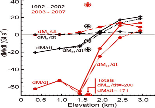
Figure 4: dM/dt is total rate of mass change, dMa/dt is the component driven by temporal variations in snow accumulation, and dMbd/dt is the component driven by ablation and ice dynamics, all averaged by 500m elevation bands over the ice sheet for the 1992–2002 and 2003–07 periods. Circled symbols are totals for all elevations weighted by area. Zwally et al., 2003
The total rate of mass change (dM/dt) was also divided into eight drainage systems (DS): two DS in the north (DS1, DS2), two in the southeast (DS3, DS4), two in the southwest (DS5, DS6) and two in the west (DS7, DS8) of Greenland (Figure 5). This provides an insight into regional differences in ice mass change.
Dynamic-/ablation-driven thinning was proven to be largest in DS3, DS4 and DS8 and very small in DS1, DS2, DS5 and DS6. Accumulation-driven mass increases are largest in DS3, DS4, DS7 and DS8.
The data used in this study was generated with the use of satellites. The ICEsat data ranges from 2003 till 2007 because during this period the satellite has been operational. The data is downloadable free of charge from the website of the National Snow and Ice Center (www.NSIDC.org). The ERS data is available on the European Space Agency website (http://earth.esa.int) although creating a free account is necessary for retrieving the data.
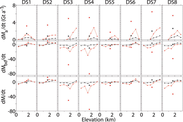
Figure 5: Components of mass change by drainage system. dMa/dt, dMbd/dt, dM/dt (Gt a–1) averaged over 500m elevation bands for the eight drainage systems for 1992–2002 (black) and 2003–07 (red) with totals for 1992–2002 (black symbols) and 2003–07 (red symbols). Zwally et al., 2003
Climate data
In a paper by Hanna et al., 2011, the mass balance of the Greenland ice sheet was constructed with the use of climate data. The reconstruction of the Greenland Ice Sheet surface mass balance (SMB) used data from 1870 to 2010 and was based on merged Twentieth Century Reanalysis (20CR) and European Centre for Medium-Range Weather Forecasts (ECMWF) meteorological reanalyses. The data used by Hanna et al. (2011) can be downloaded free of charge on the website of the National Oceanic and Atmospheric Administration (www.esrl.noaa.gov) and the website of ECMWF (www.ecmwf.int) The new SMB series was validated with global and regional climate and atmospheric circulation indices during this period. Figure 6 shows two figures, both depicting the change in surface ice mass per year, one over 40 years and the other over 20 years.
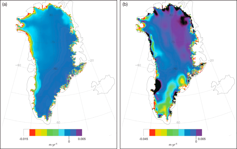
Figure 6: Linear least squares regression trends of Greenlands ice sheet surface mass balance for (a) 1870–2010 and (b) 1990–2010. Note the different scales and regional/temporal disparities of change. (Hanna et al., 2011)
Data use, availability and gaps
A time series with the changes in mass of the Greenland ice sheet was easily found. Multiple websites have interactive tools to show the Greenland ice mass over the course of time. The most prominent webpages are:
However, these tools are all based on the GRACE satellite data, which ranges from 2002 to present. Other data regarding ice mass can be found in scientific papers, but these require more effort to find, to read and to check for relevance. The data found in the scientific papers do not show actual timelines but show comparisons between averages or use cumulative depictions of ice mass change. This data does range further back in time; an average of 1992 until 2002 and 1870 (e.g. Hanna et al., 2011). The data sets used by the papers are all available free of charge, however this data is heavily processed for it to be used for expressing Greenland Ice Sheet mass balance. Therefore, specialist knowledge is required to expand the existing information regarding the ice sheet mass when using these data sets.
The websites where the data sets can be downloaded are:
- www.NSIDC.org (GRACE & ICEsat)
- https://earth.esa.int (ERS)
- www.esrl.noaa.gov (20CR)
- www.ecmwf.int (ECMWF)
Conclusion and lessons learned
This challenge was to present a time series showing the mass of ice lost from Greenland. This data is readily available with easy and free access. The data shows that the mass balance of the Greenland ice sheet is a complex system which has strong regional differences. Lessons learned are:
- The GRACE satellite dataset is the only dataset which is translated into a timeseries.
- When searching for Greenland ice mass change most information found is based on the GRACE satellite data.
- Because the only time series is derived from the GRACE dataset the time period only ranges back to 2002.
- Other depictions of ice mass variation are either comparative or cumulative.
Recommendations
When interested in the change in mass of the Greenland ice sheet not all data is equally accessible. This might result in a skewed image of the process. Creating a platform where all data is depicted might provide a more complete image. When possible, a model in which all current data and knowledge regarding the Greenland ice mass temporal change can be incorporated and be plotted over time would give the most complete image.
References:
- Barletta, V. R., Sørensen, L. S., & Forsberg, R. (2013). Scatter of mass changes estimates at basin scale for Greenland and Antarctica. The Cryosphere, 7, 1411–1432. https://doi.org/10.5194/tc-7-1411-2013
- Cuffey, K. M., & Marshall, S. J. (2000). Substantial contribution to sea-level rise during the last interglacial from the Greenland ice sheet. Nature, 404, 591. Retrieved from http://dx.doi.org/10.1038/35007053
- Gregory, J. M., Huybrechts, P., & Raper, S. C. B. (2004). Climatology: Threatened loss of the Greenland ice-sheet. Nature, 428(6983), 616.
- Hanna, E., Huybrechts, P., Cappelen, J., Steffen, K., Bales, R. C., Burgess, E., … Savas, D. (2011). Greenland Ice Sheet surface mass balance 1870 to 2010 based on Twentieth Century Reanalysis, and links with global climate forcing. JOURNAL OF GEOPHYSICAL RESEARCH, 116. https://doi.org/10.1029/2011JD016387
- Hanna, E., Huybrechts, P., Steffen, K., Cappelen, J., Huff, R., Shuman, C., … Griffiths, M. (2008). Increased Runoff from Melt from the Greenland Ice Sheet: A Response to Global Warming. Journal of Climate, 21(2), 331–341. https://doi.org/10.1175/2007JCLI1964.1
- Lenton, T. M., Held, H., Kriegler, E., Hall, J. W., Lucht, W., Rahmstorf, S., & Schellnhuber, H. J. (2008). Tipping elements in the Earth’s climate system. Proceedings of the National Academy of Sciences, 105(6), 1786–1793.
- Nghiem, S. V, Hall, D. K., Mote, T. L., Tedesco, M., Albert, M. R., Keegan, K., … Neumann, G. (2012). The extreme melt across the Greenland ice sheet in 2012. Geophysical Research Letters, 39(20), n/a--n/a. https://doi.org/10.1029/2012GL053611
- Tedesco, M., Box, J. E., Cappelen, J., Fausto, R. S., Fettweis, X., Hansen, K., … Wahr, J. (2015). Greenland Ice Sheet.
- Zwally, H. J., Li, J., Brenner, A. C., Beckley, M., Cornejo, H. G., Dimarzio, J., … Wang, W. (2003). Greenland ice sheet mass balance: distribution of increased mass loss with climate warming. Retrieved from https://icesat4.gsfc.nasa.gov/cryo_data/publications/ZwallyETALJGlac2011Jan.pdf
Traditional way of life
Quick links to:
- How is the Arctic climate changing?
- Traditional way of life
- Effects of climate change on the traditional way of life
- The migratory behaviour of caribou
- Bowhead whale
- Data use, availability and gaps
- Conclusion and lessons learned
- Lessons learned
- Recommendations
- References
Sub-challenge: observed changes in migrations and other animal behaviour relevant to traditional way of life (reindeer husbandry, whaling, fishing)
Results
Climate change can have both direct and indirect effects on the natural environment. Rising (sea) temperatures or melting sea-ice can be seen as direct effects, whereas ecological systems including (human) behaviour can be affected indirectly. Polar regions show results of climate change at a much faster pace than other regions will (Berkes & Jolly, 2001, Hobbie et al., 2017). This makes the Arctic an ideal study environment for assessing effects of climate change, including the effects on (human) behaviour. However, before we can study the impact of climate change on the traditional way of life of humans, we first need to study climate change in the Arctic, the ‘traditional way of life’ and the animals related to this.
How is the Arctic climate changing?
The Arctic climate has two main patterns of circulation (Figure 1). In the positive phase, cold air is kept within the Arctic, which is favourable for sea ice formation and associated ecosystems (Thompson and Wallace, 1998). More recently the negative phase is getting increasingly common, leading to more snow in the mid-latitude North America, Europe and eastern Asia. With more cold air escaping the Arctic, the Arctic itself warms up and sea-ice retreats and the length of open water periods in the Beaufort and Chukchi Seas is increasing (Thomson et al, 2016).
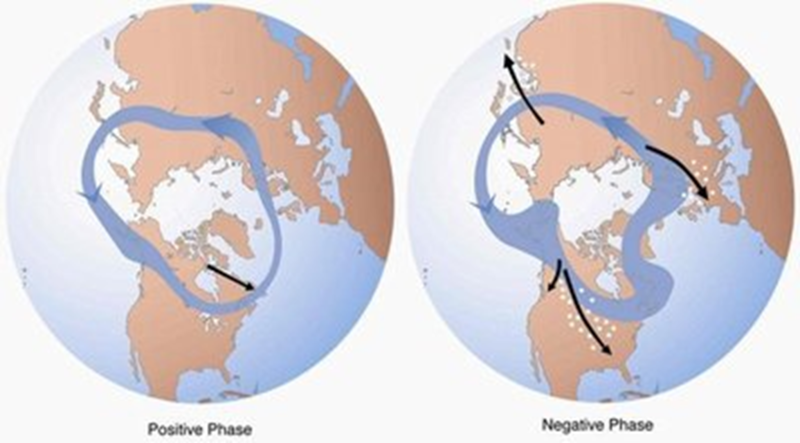
Figure 1: Different phases of the Arctic Oscillation, associated with different winds and storm tracks in the Arctic. Positive phase on the left, negative phase on the right. Courtesy of Dr. Dave Thomson, Colorado State University.
The length of the melt season in the Arctic has increased approximately by one day every two years since 1979 (Stroeve et al, 2014, see also Markus et al 2009). As open water absorbs more solar radiation than ice cover, sea surface temperature (SST) in the Arctic has increased by 0.5-1.5?C over the last decade (see also the Temperature sub-challenges), leading to delays in the timing of freeze-up initiation (Markus et al, 2009). This has resulted in changes in the overall ice thickness of Arctic sea ice (Animations of changing sea ice export and ice thickness are available from NASA Goddard's Scientific Visualization Studio: https://www.nasa.gov/feature/goddard/2016/arctic-sea-ice-is-losing-its-bulwark-against-warming-summers). Timing of migratory species has changed with the sea ice, e.g. the autumn migration of Beluga whales has delayed an average of 4 days/year, based on data from 2008-2014 (Hauser et al, 2016).
Traditional way of life
The ‘traditional way of life’ can be linked to indigenous people, keeping to traditions set many generations ago, often making use of subsistence herding, gathering, hunting or fishing. During the last century, Arctic regions have modernized enormously. For example, in Greenland subsistence hunting and fishing is still widespread, but it has increasingly become a leisure activity in comparison to a ‘way of life’ (Curtis et al. 2005). A similar change can be found in Northern Siberia (Koptseva & Kirko, 2014), Alaska (Moerlein & Carothers, 2012), as well as in the far north of Canada (Berkes & Jolly, 2001; Searles, 2008), where supermarkets and imported foods now add to the diet collected by traditional gathering and hunting (Lougheed, 2010). For this study, no distinction is made between people fully depending on a subsistence way of life, partly depending on it, or not depending on it but still using it for traditional or other purposes.
Because of modernization, social, economic, and demographic change, as well as resource development, trade barriers and animal-rights movements, there have been many changes in human behaviour with regards to the ‘traditional way of life’ (Nuttall et al., 2005). It is hard to filter out which change led to which effect, as many of the changes link together and influence each other.
Effects of climate change on the traditional way of life
Climate change can affect species used for subsistence, but it also affects the means of gathering them. For example, summer sea-ice retreat can lead to a smaller hunting area, extreme weather can damage village infrastructure, melting permafrost can lead to altered spring run-off patterns and changing sea levels and tidal fluctuations can pose dangerous fishing conditions. Unpredictable weather due to climate change has impact on many aspects, as shown in Figure 3.
The impact of climate change on traditional life is not always linear, it can be a complex network of relationships and effects, each in turn connected to many other aspects. For example, due to the rapid changes in climate, elders are unable to predict weather compared to their former knowledge and experience, and they cannot pass this knowledge on to the next generation. Lower predictive skill means increased risks of failure or accidents during hunting, migration, food collection and camp formation. Loss of these traditional skills changes the way of life rapidly. Efforts to map traditional knowledge in peer reviewed scientific studies have been limited in success due to the difference in the types of information: historical knowledge and experience vs. experimental or observational studies.
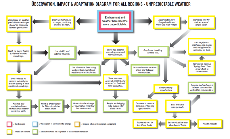
Figure 3: Observation, impact & adaptation diagram for Canadian Inuit regions on unpredictable weather. Source: Nickels et al. 2005.
Fish is the most reliable subsistence resource in Alaska (Moerlein & Carothers, 2012). In several communities in north-western Alaska the catch contains chum salmon (Oncorhynchus keta), dolly varden (Salvelinus malma) and several species of whitefish (Moerlein & Carothers, 2012). Fishing and hunting practices are extremely flexible in response to changing conditions and needs (Moerlein & Carothers, 2012).
Musk-ox (Ovibos moschatus), lesser snow goose (Anser caerulescens), ringed seal (Phoca hispida), and various fish species are the main species for hunting in the Canadian Arctic (Berkes & Jolly, 2001). During winter, people hunt musk-ox and, to a lesser extent, caribou (Rangifer tarandus), arctic foxes (Alopex lagopus), wolves (Canis lupus), polar bears (Ursus maritimus), and ringed seals (Pusa hispida). The study provides a list of examples of local environmental changes and effects on subsistence activity described by members of the community. This includes impacts on access, safety, predictability and species availability. For example, old ice doesn't come in close to the settlement in summer anymore which makes it more difficult to hunt seals; open sea-ice in winter makes travel dangerous; the arrival of spring differs from year to year; and more rain in the fall increases chances of freezing rain, which can lead to caribou starving. The effects of these changes and the response strategies of the affected people vary. Because of modernisation most communities have a wider range of food options now, making it less vital for a direct need to adapt to the environmental changes. Response strategies on a short-term such as use of other vehicles for travel, changing hunting areas or waiting for the appropriate timing are applied (Berkes & Jolly, 2001). Long-term adaption strategies are only speculated. Climate Change may not always have a negative effect. For example, with seawater temperatures rising, marine fishes of a more temperate origin move northward into the Arctic seas (Christiansen, Mecklenburg, & Karamushko, 2014). Two species of Pacific Salmon were welcomed by local inhabitants.
A combination of modernisation, globalisation and Climate Change has affected subsistence living conditions in Upernavik in northern Greenland (Hendriksen & Jørgensen, 2015). Since the 1980s Greenland Halibut fishing in dinghies has been a major source of income for the local community in summer. Dangerous situations arise when the shorter period of sea-ice forces fishing to be carried out in the dark winter period as well. The same applies for hunting of whales and seals. Local communities have been rather resilient and adaptive in meeting the challenges set by Climate Change, due to their traditional and local knowledge (Hendriksen & Jørgensen, 2015). They point out that governance (such as restrictions in hunting or fishing methods or set quotas) is even more challenging than the changes in their natural environment; it is not only Climate Change which threatens the traditional way of life.
The migratory behaviour of caribou
Distribution and ecology
Caribou (Rangifer tarandus) is a species of deer native to the Arctic environment. There are many subspecies within the circumpolar distribution (see Figure 4). Some of the populations are sedentary while others are typically migratory. Caribou are unique ruminants, feeding mainly on lichens and some senescent browse in wintertime (Parker et al. 2005).
An interactive map with caribou habitats can be found here: http://carma.caff.is.
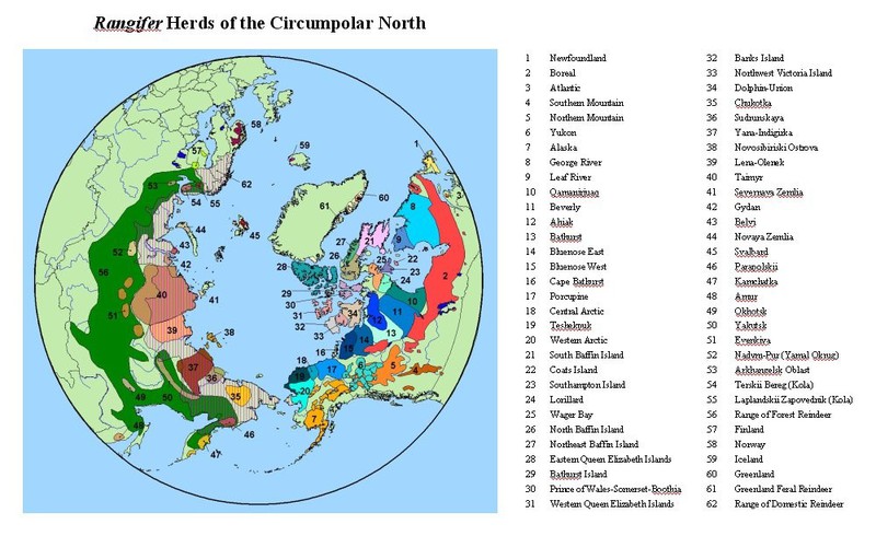
Figure 4: Circumpolar distribution of reindeer and caribou with associated population names. Source: CARMA https://www.caff.is/images/_Organized/CARMA/Welcome_to_CARMA/Map/Circumpolar%20herds.jpg accessed on April 25th, 2017).
The species Rangifer tarandus is called ‘reindeer’ in Europe and Asia and ‘caribou’ in North America. However, there seems to be genetic diversity between the two, with two original lineages: one originating from and confined to Northeastern America, and the other originating from Euro-Beringia but also currently distributed in western North America (Yannic et al. 2013). For this report however, no distinction is made between the two and Rangifer tarandus is used for both caribou and reindeer and ‘caribou’ is used to indicate Rangifer tarandus.
Effects of Climate Change of caribou
Climate Change can impact caribou in many ways. For example through changes in habitat and food accessibility, and in temperature, see Table 1 (source: CARMA, CircumArctic Rangifer Monitoring and Assessment Network, accessed on April 11, 2017).
Table 1: Climate Change impacts on caribou. Source: http://carma.caff.is
| Climate Change Condition | Impact on Habitat | Impact on Movement | Impact on Body Condition | Impact on Productivity | Management Implications |
| Earlier snowmelt on coastal plain | Higher plant growth rate | Core calving grounds move further north Less use of current calving grounds | Cows replenish protein reserves faster Higher calf growth rate | Higher probability of pregnancy Higher June calf survival | Need for wider calving ground protection |
| Warmer, drier summer | Earlier peak biomass Plants harden earlier Reduction in mosquito breeding sites Increased oestrid harassment Increased frequency of fires on winter range Fewer “mushroom” years | Movement off of calving grounds earlier More use of insect relief habitat in July Avoidance of recently burned winter habitat | Increased harassment will lower fall body condition | Reduced probability of pregnancy | Protection of insect relief areas important |
| Warmer, wetter fall | More frequent icing conditions | Caribou abandon ranges with severe surface icing | Higher winter mortality Earlier weaning | ||
| Warmer, wetter winters | Deeper denser snow Icing conditions, especially in tundra and arctic islands | Increased dependence on low snow regions stay on winter range longer | Greater over winter weight loss higher incidence of extended lactation | lower over winter mortality on calves | Need to consider protection of low snow regions |
| Warmer springs | More freeze/thaw cycles during spring migration Faster spring melt | Movement slowed and/or movement unto drier windswept ridges | Accelerated weight loss in spring | Higher wolf predation on cows and calves due to use of windswept ridges | Concern over timing and location of spring migration in relation to traditional harvesting areas |
|
Overall Effect: In very general terms the calving range improves but movement and reliance on more northern portions of the calving range; animals leave calving range earlier; cows and calves suffer reduced summer and autumn body reserves due to increase in oestrid fly harassment; mosquito harassment may be reduced if summers are drier; more frequent icing on autumn, winter and spring ranges which, depending on the location of these ranges may have moderate to severe implications to body condition and survival. In relation to management, there will be an overall need to assess habitat protection in relation to climate trends, need to factor climate change impacts on harvest strategy, need to communicate impacts of climate on harvest patterns and timing and a need to set up comprehensive monitoring programs. |
|||||
Behaviour of two herds of caribou in Canada is described as: “Migratory caribou appeared to prefer regions with higher snowfall and lichen availability in the fall and winter. In the summer, caribou preferred cooler areas likely corresponding to a lower prevalence of insects, and they avoided disturbed and recently burnt areas (Sharma et al. (2009).” Models were used to indicate possible responses of these herds to Climate Change. The results are variable, as responses depend on the current migratory pattern and habitats and the possible effect of Climate Change in this. This limits the range of one herd but increases the range of the other, limiting both to a certain region (Sharma et al. 2009).
Influence of climate change on the behaviour of caribou and the traditional way of life
Caribou are an important source of food in the traditional way of life all over the Arctic. Impacts of climate change on the traditional way of life can include the loss of possible hunting areas or herds either in certain periods of time or permanently, as well as the other way around. Freezing rain in fall can lead to caribou starvation which would lead to a lower prey availability for subsistence hunting (Berkes & Jolly, 2001). On the contrary, increased availability of summer forage and more wind as favourable conditions may lead to a higher prey availability.
Traditional knowledge gives subsistence hunters flexibility in dealing with climate change (Pearce et al., 2015). For example, knowledge of caribou husbandry but also knowledge on how to deal with and prepare for hazardous hunting conditions can give the hunters footholds when conditions change.
In conclusion, climate change has a direct effect on caribou behaviour which in turn influences the traditional way of life. However, effects of climate change on caribou are variable, resulting in both positive and negative effects for subsistence hunters. The effects depend on (among others) location and normal migration behaviour of the caribou, season, and (traditional) knowledge and flexibility of the hunters.
Bowhead whale
Distribution and ecology
Bowhead whales (Balaena mysticetus) typically live in the Arctic and are divided in four stocks: Bering-Chukchi-Beaufort Seas (US (Alaska), Canada, and Russian Federation); eastern Canada – west Greenland (Canada and Denmark (Greenland)); Svalbard-Barents Sea (Spitsbergen) (Denmark (Greenland), Norway, and Russian Federation); and the Okhotsk Sea (Russian Federation and Japan) (COSEWIC, 2009; Reilly et al. 2012). The eastern Canada – west Greenland stock was previously thought to be two separate stocks (Hudson Bay-Foxe Basin; Davis Strait-Baffin Bay), however new research showed they belong to the same stock (COSEWIC, 2009; Wiig et al. 2009).
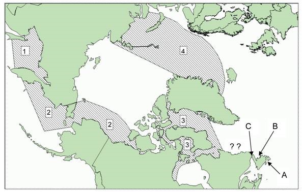
Figure 5: Four different stocks of the Bowhead Whale. 1. Okhotsk Sea, 2. Bering–Chukchi–Beaufort seas (BCB DU), 3. Eastern Canada – West Greenland (EC–WG DU), 4. Svalbard/Barents Sea. Question marks denote the Labrador coast where Inuit are historically reported to have harvested Bowheads. Basque whalers hunted Bowheads in the Strait of Belle Isle (C). Floating or stranded Bowhead carcasses were observed at Rattling Brook (B) in 1998 and Mobile Point (A) in 2005. Source: COSEWIC, 2009.
During summertime bowhead whales migrate to the high Arctic and they retreat to the sea-ice edges during wintertime (Reilly et al. 2012). Bowhead whales are very large animals with body lengths of over 19 meter and a body mass of over 80 metric ton (George et al. 2015). Despite their size, bowhead whales feed mostly on zooplankton in the form of medium-sized crustaceans such as krill and copepods (Reilly et al. 2012).
All bowhead whale stocks have been severely overexploited during the commercial whaling periods of the 18th and 19th century. Since the end of the large-scale commercial whaling the stocks are slowly recovering. The Bering-Chukchi-Beaufort Seas (BCB) stock is thought to be close to pre-whaling levels, but the Atlantic stocks recover more slowly and are still at relatively low levels (Fauchald et al. 2017).
Effects of climate change on the bowhead whale
As bowhead whales are a typical ice-associated migratory species, climate change could have a direct effect on them. The bowhead’s food, zooplankton, is closely coupled to the primary production, which in turn is directly influenced by climate change (see also the sub-challenge ‘phytoplankton’) (George et al. 2015). However, bowhead whales are not directly dependent on the presence of sea-ice but more on the presence of zooplankton, which may also be present in open water. The reduction of sea-ice could even have a positive influence on the amount of available prey for the bowhead whale through an increase in primary production (George et al. 2015; Moore & Huntington, 2008; Moore & Laidre, 2006).
Influence of climate change on the behaviour of bowhead whales and the traditional way of life
Bowhead whales have been part of subsistence hunting for thousands of years (Ashjian et al. 2010; Seersholm et al. 2016; Suydam & George, 2004). Current subsistence hunting on bowhead whales is regulated through strict quotas to not impede further stock recovery (Fauchald et al. 2017).
Subsistence whaling in the BCB stock (Alaska) can be taken as an example. The (rough) migratory pattern of this stock is depicted in Figure 6 (George et al. 2015). During the spring and fall migrations the local communities of Northern Alaska hunt the bowhead whales to provide subsistence food (Ashjian et al. 2010). The presence of bowhead whales is mostly dependent on readily available food sources (zooplankton) which can be directly seen in its distribution.
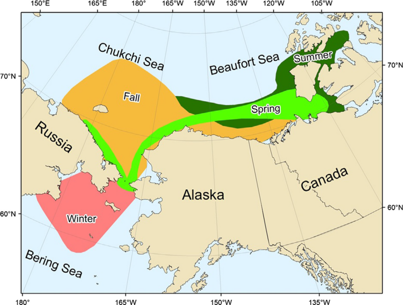
Figure 6: Seasonal range map of the Bering–Chukchi–Beaufort bowhead whales based on satellite telemetry data (Quakenbush et al., 2012). Bowheads are also known to occur in regions outside these general boundaries. Source: George et al. 2015.
Four factors influence the availability of euphausiids (krill) as food source for bowhead whales near Barrow (at the most northern tip of Alaska) during the migration seasons (Ashjian et al., 2010):
-
the northwards transport of Pacific Water during spring;
- the quantity of euphausiids in the Pacific Water and their growth and survivorship during their transit across the Chukchi Sea to the Barrow region;
- the transit time of Pacific Water and plankton from the Bering Strait to Barrow;
- the existence of mechanisms that aggregate euphausiids into dense prey patches.
All the factors link to each other and are affected by climate change effects. Certain wind conditions have influence on the upwelling and aggregation of euphausiids. This creates favourable conditions for bowhead whales and consequently for subsistence hunters. When weather and wind patterns change due to climate change, migration patterns could be altered and subsistence hunting could be affected (Ashjian et al. 2010). Considerable inter annual variation is seen in migration and summer locations of bowheads, possibly due to shifting environmental conditions (Fauchald et al. 2017). Bowhead whales arrive earlier and hunting starts earlier in spring and later in autumn (Huntington et al. 2016). Less multiyear sea-ice and thinner land-ice has made it harder to find ice floats for hauling out whales for butchering in spring. Whales no longer appear to feed along the edge of the land-ice southwest of Barrow in spring (Huntington et al. 2016). The latter seems to pose a bigger problem for the native subsistence hunters than the changing migratory patterns, as the traditional bowhead hunts rely on the presence of sea-ice (Sakakibara, 2017).
In conclusion, climate change has an effect on Bowhead whales’ migration behaviour which in turn influences the traditional way of life. However, as the bowhead whale hunt is influenced by other factors as well, some of them also dependent on climate change, there is not always a direct relationship.
Data use, availability and gaps
To provide a more in depth answer on the availability and quality of data, a more narrow and specified question is needed. For now, two species were chosen to illustrate the effects of climate change on animal behaviour and the traditional way of life. On the (migratory)behaviour of caribou and bowhead whales information can be found mainly in scientific papers published in peer-reviewed journals. Because climate change can have effects on species’ behaviour in various ways with various outcomes it was difficult to build databases for this topic. However, information on the (migratory) behaviour of specific populations or stocks of animals used for the traditional way of life and the influence of climate change on this can’t be found in a single database or data source. While it is complicated to monitor the effects of climate change on the traditional way of life, it is possible to monitor species’ migrations and/or behaviour in areas in which climate change is visible.
Conclusion and lessons learned
Climate change impacts the traditional way of life. This may be a consequence of the effect of climate change on animal behaviour such as migration routes. However, people still actively pursuing the traditional way of life in the Arctic seem to be very adaptive to changing conditions. For example, Inuit in the Canadian Arctic are very flexible, showing responses to varying climatic conditions (Figure 7, Pearce et al. (2015).
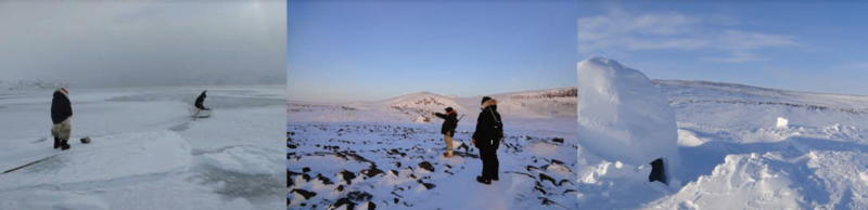
Figure 7: Photographs of Inuit in the Canadian Arctic illustrating responses to changing climatic conditions that affect subsistence. (Left): Flexibility – Iqaluit hunters improvise, using boats to maintain access to seal hunting areas in late fall. (Centre): Hazard avoidance – Ulukhaktok hunters make extra efforts to read weather and ice conditions before and during travel. (Right): Emergency preparedness – Knowledge of how to build an emergency snow house enables hunters to wait out storm events. Source: Pearce et al. 2015.
A similar optimism can be found for sustaining subsistence systems, pointing at the long history of subsistence systems and its apparent resilience (Kofinas et al., 2010). However, changing climatic conditions may prove to be too problematic for certain types of traditional hunting as simple things like access to the food source may cause a significant reduction in the availability of subsistence resources in the future (Brinkman et al. 2016).
Lessons learned
Lessons learned during the answering of this sub-challenge:
- There are many types of traditional life, with communities varying in traditions, size, etc., and information is not always available;
- Information on animal migration and the influence of climate change on migration behaviour is available for some species such as caribou and bowhead whales;
- The available information is usually in text-form as scientific published peer-reviewed papers;
- Behavioural changes and effects of climate change will not always be directly related, as complex interactions and relations can alter parts of the system or combinations of different systems;
- Databases with direct numbers are not always available;
- Climate change is not the only thing affecting the traditional way of life: globalization, westernization and modernization are only some of the other factors influencing the traditional way of life.
Recommendations
To know the needs of the people using the traditional ways of life and the influence of climate change on animal behaviour linked to this, long term and consistent research is needed. Examples of monitoring are:
- Per traditional community the most used wild species for subsistence reasons;
- Per traditional community the direct effects of climate change on the traditional way of life through subsistence hunting and fishing such as ice decline or weather changes;
- Specific species populations or stocks used for subsistence reasons;
- (Migratory) behaviour of the specific populations or stocks used for subsistence reasons;
- Effects of climate change on the habitat and (migratory) behaviour of specific populations or stocks used for subsistence reasons.
The results of the monitoring should be openly available in a public database.
- Ashjian, C. J., Braund, S. R., Campbell, R. G., GEORGE, J. C., Kruse, J., Maslowski, W., ... & Sherr, E. B. (2010). Climate variability, oceanography, bowhead whale distribution, and Iñupiat subsistence whaling near Barrow, Alaska. Arctic, 179-194. http://darchive.mblwhoilibrary.org/bitstream/handle/1912/5127/973-2855-1-PB.pdf?sequence=1
- Berkes, F., & Jolly, D. (2001). Adapting to climate change: Social-ecological resilience in a Canadian western arctic community. Conservation Ecology, 5(2), 18.
- Brinkman, T. J., Hansen, W. D., Chapin, F. S., Kofinas, G., BurnSilver, S., & Rupp, T. S. (2016). Arctic communities perceive climate impacts on access as a critical challenge to availability of subsistence resources. Climatic Change, 139(3-4), 413-427. https://static1.squarespace.com/static/542db5eae4b03f0fd61b3bb5/t/58389c79579fb36e9c8334d3/1480105095696/
brinkman+et+al.+2016.pdf - COSEWIC. 2009. COSEWIC assessment and update status report on the Bowhead Whale Balaena mysticetus, Bering–Chukchi–Beaufort population and Eastern Canada–West Greenland population in Canada. Committee on the Status of Endangered Wildlife in Canada. Ottawa. vii + 49 pp. http://www.sararegistry.gc.ca/default.asp?lang=En&n=082503B1-1
- Curtis, T., Kvernmo, S., & Bjerregaard, P. (2005). Changing Living Conditions. International Journal Of Circumpolar Health, 64(5), 442–450. Retrieved from http://scholar.google.nl/scholar_url?url=http://journals.co-action.net/index.php/ijch/article/download/18025/20515&hl=nl&sa=T&oi=gga&ct=gga&cd=28& ei=qLMEV6esCYGTmgHoyKeQDg&scisig=AAGBfm2dQXvSs6B7HVtOYa8irnMMkP2xxw&nossl=1&ws=1280x843
- Fauchald, P., Hausner, V., Schmidt, J., & Clark, D. (2017). Transitions of social-ecological subsistence systems in the Arctic. International Journal of the Commons, 11(1). https://www.thecommonsjournal.org/articles/10.18352/ijc.698/
- George, J. C., Druckenmiller, M. L., Laidre, K. L., Suydam, R., & Person, B. (2015). Bowhead whale body condition and links to summer sea ice and upwelling in the Beaufort Sea. Progress in Oceanography, 136, 250-262. http://faculty.washington.edu/klaidre/docs/George%20et%20al.%202015.pdf
- Hauser, D. D., Laidre, K. L., Stafford, K. M., Stern, H. L., Suydam, R. S., & Richard, P. R. (2017). Decadal shifts in autumn migration timing by Pacific Arctic beluga whales are related to delayed annual sea ice formation. Global change biology, 23(6), 2206-2217.
- Hendriksen, K., & Jørgensen, U. (2015). Hunting and fishing settlements in Upernavik district of Northern Greenland – challenged by climate, centralization, and globalization. Polar Geography, 38(2), 123–145. http://doi.org/10.1080/1088937X.2015.1034222
- Hobbie, J.E., Shaver, G.R., Rastetter, E.B., Cherry, J.E., Goetz, S.J., Guay, K.C, Gould, W.A. & Kling, G.W. (2017). Ambio 46 (Suppl 1): 160. https://doi.org/10.1007/s13280-016-0870-x
- Huntington, H. P., Quakenbush, L. T., & Nelson, M. (2016). Effects of changing sea ice on marine mammals and subsistence hunters in northern Alaska from traditional knowledge interviews. Biology Letters, 12(8), 20160198. http://rsbl.royalsocietypublishing.org/content/roybiolett/12/8/20160198.full.pdf
- Kofinas, G. P., Chapin, F. S., BurnSilver, S., Schmidt, J. I., Fresco, N. L., Kielland, K., ... & Rupp, T. S. (2010). Resilience of Athabascan subsistence systems to interior Alaska’s changing climate This article is one of a selection of papers from The Dynamics of Change in Alaska’s Boreal Forests: Resilience and Vulnerability in Response to Climate Warming. Canadian Journal of Forest Research, 40(7), 1347-1359. https://www.fs.fed.us/pnw/pubs/journals/pnw_2010_kofinas001.pdf
- Koptseva, N. P., & Kirko, V. I. (2014). Ethic identification of indigenous people of the Siberian Arctic. American Journal of Applied Sciences, 11(9), 1573-1577.
- Lougheed, T. (2010). The Changing Landscape of Arctic Traditional Food. Environmental Health Perspectives, 118(9), a386–a393. https://ehp.niehs.nih.gov/118-a386/
- Markus, T., Stroeve, J. C., & Miller, J. (2009). Recent changes in Arctic sea ice melt onset, freezeup, and melt season length. Journal of Geophysical Research: Oceans, 114(C12). http://onlinelibrary.wiley.com/doi/10.1029/2009JC005436/epdf
- Moerlein, K. J., & Carothers, C. (2012). Total Environment of Change: Impacts of Climate Change and Social Transistions on Subsistence Fisheries in Northwest Alaska. Ecology and Society, 17(1), 10. https://www.ecologyandsociety.org/vol17/iss1/art10/
- Moore, S. E., & Huntington, H. P. (2008). Arctic marine mammals and climate change: impacts and resilience. Ecological Applications, 18(sp2). http://www.westcoast.fisheries.noaa.gov/publications/protected_species/marine_mammals/cetaceans/gray_whales/ studies_under_review/moore_and_huntington_2008.pdf
- Moore, S. E., & Laidre, K. L. (2006). Trends in sea ice cover within habitats used by bowhead whales in the western Arctic. Ecological Applications, 16(3), 932-944. https://staff.washington.edu/klaidre/docs/MooreandLaidre_2006.pdf
- Nicholson KL, Arthur SM, Horne JS, Garton EO, Del Vecchio PA (2016). Modeling Caribou Movements: Seasonal Ranges and Migration Routes of the Central Arctic Herd. Welker JM, ed. PLoS ONE. 2016;11(4):e0150333. http://journals.plos.org/plosone/article?id=10.1371/journal.pone.0150333
- Nickels, S., Furgal, C., Buell, M.& Moquin, H. (2005). Unikkaaqatigiit – Putting the Human Face on Climate Change: Perspectives from Inuit in Canada. Ottawa: Joint publication of Inuit Tapiriit Kanatami, Nasivvik Centre for Inuit Health and Changing Environments at Université Laval and the Ajunnginiq Centre at the National Aboriginal Health Organization. 129p. https://www.itk.ca/wp-content/uploads/2016/07/unikkaaqatigiit01-1.pdf
- Nuttall, M., Berkes, F., Forbes, B., Kofinas, G., Vlassova, T., & Wenzel, G. W. (2005). Hunting, herding, fishing, and gathering: Indigenous peoples and renewable resource use in the Arctic. In Arctic Climate Impact Assessment (pp. 649–690). New York, NY, USA: Cambridge University Press. Retrieved from http://www.acia.uaf.edu/PDFs/ACIA_Science_Chapters_Final/ACIA_Ch12_Final.pdf
- Parker, K. L., Barboza, P. S., & Stephenson, T. R. (2005). Protein conservation in female caribou (Rangifer tarandus): effects of decreasing diet quality during winter. Journal of Mammalogy, 86(3), 610-622. http://web.unbc.ca/~parker/Pubs/ParkerBarbozaStephenson%202005JMamm.pdf
- Pearce, T., Ford, J., Willox, A. C., & Smit, B. (2015). Inuit traditional ecological knowledge (TEK), subsistence hunting and adaptation to climate change in the Canadian Arctic. Arctic, 233-245. http://arctic.journalhosting.ucalgary.ca/arctic/index.php/arctic/article/download/4475/4592
- Quakenbush, L., Citta, J., George, J. C., Heide-Jørgensen, M. P., Small, R., Brower, H., ... & Pokiak, C. (2012). Seasonal movements of the Bering-Chukchi-Beaufort stock of bowhead whales: 2006–2011 satellite telemetry results. Int Whal Comm Sci Report SC/64/BRG1. http://www.north-slope.org/assets/images/uploads/SC-64-BRG1.quakenbush_et_al.2012.pdf
- Reilly, S.B., Bannister, J.L., Best, P.B., Brown, M., Brownell Jr., R.L., Butterworth, D.S., Clapham, P.J., Cooke, J., Donovan, G., Urbán, J. & Zerbini, A.N. 2012. Balaena mysticetus. The IUCN Red List of Threatened Species 2012: e.T2467A17879018. http://dx.doi.org/10.2305/IUCN.UK.2012.RLTS.T2467A17879018.en. Downloaded on 11 April 2017.
- Sakakibara, C. (2017). People of the Whales: Climate Change and Cultural Resilience Among Iñupiat of Arctic Alaska. Geographical Review, 107(1), 159-184. http://onlinelibrary.wiley.com/doi/10.1111/j.1931-0846.2016.12219.x/epdf
- Searles, E. N. (2008). Inuit identity in the Canadian Arctic. Ethnology, 47(4), 239–255. http://134.82.10.249/Documents/SociologyAnthropology/Inuit%20Identity%20in%20the%20Canadian%20Arctic[1].pdf
- Seersholm, F. V., Pedersen, M. W., Søe, M. J., Shokry, H., Mak, S. S. T., Ruter, A., ... & Meldgaard, M. (2016). DNA evidence of bowhead whale exploitation by Greenlandic Paleo-Inuit 4,000 years ago. Nature Communications, 7. https://www.ncbi.nlm.nih.gov/pmc/articles/PMC5105157/
- Sharma, S., S. Couturier & S.D. Côté, 2009. Impacts of climate change on the seasonal distribution of migratory caribou. Global Change Biology 15(10): 2549-2562. http://onlinelibrary.wiley.com/doi/10.1111/j.1365-2486.2009.01945.x/abstract
- Stroeve, J. C., Markus, T., Boisvert, L., Miller, J., & Barrett, A. (2014). Changes in Arctic melt season and implications for sea ice loss. Geophysical Research Letters, 41(4), 1216-1225. http://onlinelibrary.wiley.com/doi/10.1002/2013GL058951/full
- Suydam, R. S., & George, J. C. (2004). Subsistence harvest of bowhead whales (Balaena mysticetus) by Alaskan Eskimos, 1974 to 2003. Unpublished Report SC/56/BRG12. Cambridge, UK: IWC. http://www.north-slope.org/assets/images/uploads/1974-2003%20Village_harv%20BRG12.pdf
- Thomson, J., Fan, Y., Stammerjohn, S., Stopa, J., Rogers, W. E., Girard-Ardhuin, F., ... & Ackley, S. (2016). Emerging trends in the sea state of the Beaufort and Chukchi seas. Ocean Modelling, 105, 1-12. http://www.sciencedirect.com/science/article/pii/S1463500316300622
- Thompson, D. W., & Wallace, J. M. (1998). The Arctic Oscillation signature in the wintertime geopotential height and temperature fields. Geophysical research letters, 25(9), 1297-1300. http://onlinelibrary.wiley.com/doi/10.1029/98GL00950/pdf
- Wiig, Ø., Bachmann, L., Heide-Jørgensen, M. P., Laidre, K. L., Postma, L. D., Dueck, L., & Palsbøll, P. J. (2010). Within and between stock re-identifications of bowhead whales in Eastern Canada and West Greenland. Rep Int Whal Comm SC62/BRG65. https://www.researchgate.net/profile/Mads_Peter_Heide-Jorgensen/publication/242554307_Within_and_between_stock_re-identifications_of_bowhead_whales_in_Eastern_Canada_and_West_Greenland/links/0a85e52de97bf8f101000000.pdf
- Yannic, G., Pellissier, L., Ortego, J., Lecomte, N., Couturier, S., Cuyler, C., ... & Kolpashikov, L. (2014). Genetic diversity in caribou linked to past and future climate change. Nature Climate Change, 4(2), 132-137.
Abundance of three most abundant species of phytoplankton expressed as time series
Results
The definition of plankton is a group of organisms in aquatic environments which are carried along by ocean currents without the means to swim against them. Phytoplankton are the ‘flora’ plankton, or microalgae, and contain chlorophyll for photosynthesis. Primary production in oceans can be measured through chlorophyll concentrations, however this measurement does not distinguish between different species of phytoplankton. Dinoflagellates and diatoms are the two most common classes of phytoplankton.
In the Arctic area, phytoplankton are essential for primary production and serve as the basis of the marine food web. Both the presence of nutrients and light availability limit primary production, giving the Arctic area a distinct seasonal character. Upwelling of warm nutrient-rich Atlantic Water is one of the key factors driving primary production.
As described in Hallegraeff (2010): “Climate change confronts marine ecosystems with multifactorial stressors, such as increased temperature, enhanced surface stratification, alteration of ocean currents, intensification or weakening of nutrient upwelling, stimulation of photosynthesis by elevated CO2, reduced calcification from ocean acidification, and changes in land runoff and micronutrient availability”. Because climate change does not affect the phytoplankton habitat in a singular way, it is difficult to predict the response of the phytoplankton community. For example, the winter sea-ice decline creates favourable conditions for upwelling, creating in turn favourable conditions for phytoplankton (Falk-Petersen et al., 2015). Other studies however indicate a less favourable condition for phytoplankton through freshening of the water by melting ice (Coupel et al., 2015). Larsen et al. (2014) indicate that decreased sea-ice is associated with earlier phytoplankton blooms. It is clear however, that the declining sea-ice extent in the Arctic area is contributing to shifts in primary production (Frey, Moore, Cooper, & Grebmeier, 2015; Logvinova, Frey, Mann, Stubbins, & Spencer, 2015). In 2011, NOAA published a map showing the change in primary productivity, based on a study by Arrigo & van Dijken (2015), see Figure 1.
Higher ocean temperatures create an increasingly stratified water column, inhibiting nutrient rich waters from mixing with nutrient depleted waters. The quantity of larger phytoplankton such as diatoms are predicted to decrease as they need more nutrients to survive, compared with smaller phytoplankton such as cyanobacteria (Lindsey & Scott, 2010). However, in the polar regions the reduced mixing will keep the plankton closer to the surface (and to sunlight), creating favourable conditions for an increase in plankton (Hallegraeff, 2010). In general, the effects of Climate Change on phytoplankton is poorly understood (Hoppe et al., 2016).
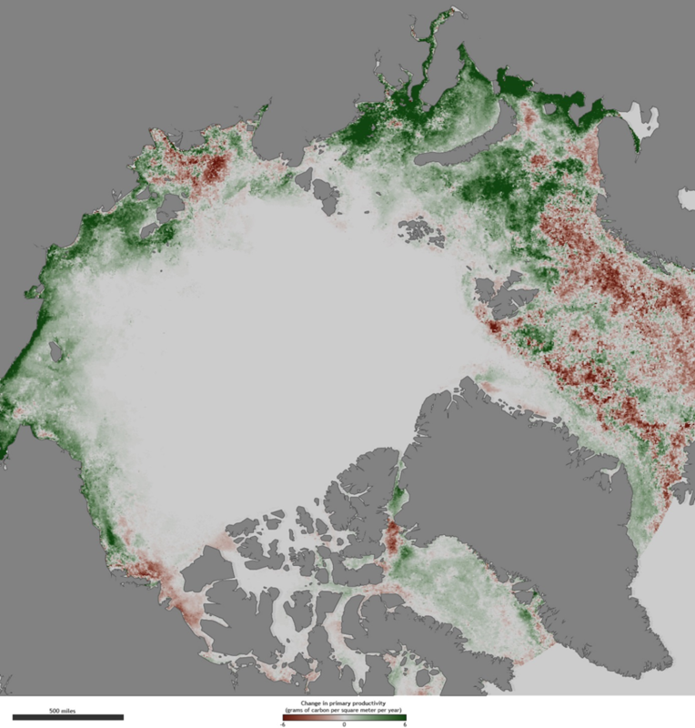
Figure 1: Changes in primary production between 1998 and 2000. Browns show declines, while greens show increases. Increases in primary production were greatest in the eastern Arctic Ocean, mirroring the areas of greatest sea ice loss in the Kara and East Siberian seas (source: Arrigo & van Dijken 2011 and NOAA 2011).
As can be seen in Figure 1, the primary production varies over the entire Arctic area, even over a limited time span of two years.
The COPEPOD database has a nice summary of available plankton data in the Arctic area. https://www.st.nmfs.noaa.gov/copepod/content/region_arctic.html. COPEPOD stands for ‘The Coastal & Oceanic Plankton Ecology, Production & Observation Database’ and is an online database of plankton abundance, biomass, and composition data compiled from a global assortment of cruises, projects, and institutional holdings. It was created by NOAA's National Marine Fisheries Service. Full database content and method summaries are released roughly every few years (e.g. COPEPOD-2014, COPEPOD-2010, COPEPOD-2007, COPEPOD-2005), with new data content added and immediately available online each month. COPEPOD has an interactive map area for phytoplankton, as shown as a screenshot in Figure 2.
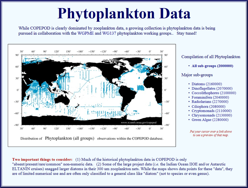
Figure 2: Phytoplankton data in COPEPOD. (http://www.st.nmfs.noaa.gov/copepod/atlas/index-atlas.html#phytoplankton)
As can be seen on the screenshot, the phytoplankton data available is quite limited. All data from COPEPOD can be downloaded and viewed in different images, such as per sub-group or season. The data downloaded from COPEPOD is a compilation of all known phytoplankton data. When only the data from a Latitude of 60 and up are shown, 42747 data points remain, showing data between 1913 to 2015 (this can be downloaded as Excel file). However, as this data is not consistent in time and space, or even in monitoring effort on the same points), creating time series would not deliver consistent images. In total, 834 species are listed in this data set, with Thalassiosira gravida, Nitzschia longissima en Protoperidinium pellucidum counting the most points.
As an example, from the Biological Atlas of the Arctic Seas 2000 (BAAS2000): Phytoplankton data was downloaded from COPEPOD for 158 scientific cruises in the Barents and Kara Seas in the period 1913 - 1999 (part of NOAA, https://www.nodc.noaa.gov/OC5/BARPLANK/start.html). The most abundant species in this data set were: Fragilaria spp, Thalassiosira spp, Chlorophycota spp, Nitzschia spp and Melosira spp. However, due to the spatial and temporal gaps in the data, it is not suitable to create time series. On the website of BAAS2000, there is a small section on changes in the phytoplankton community over time. Three options are available: 1921 vs. 1997 Barents Sea, 1921-1957-1985-1997 Barents Sea and 1921 vs. 1997 Kola Section. When clicking on this, information on the data and some figures come up, as in Figure 3.
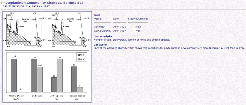
Figure 3: Screenshot of the BAAS2000 phytoplankton community changes website (https://www.nodc.noaa.gov/OC5/BARPLANK/WWW/HTML/phyt_ch1.html).
COPEPODITE is a branch from COPEPOD; an interactive time-series explorer analysis toolkit and metabase (http://www.st.nmfs.noaa.gov/copepodite/index.html). It provides a map overview of global monitoring, with clickable monitoring points. As an example, we chose the Siglunes Transect north of Iceland (Figure 4).
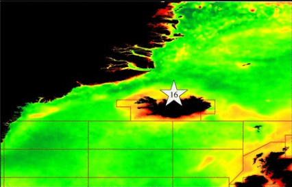
Figure 4: Location of Siglunes Transect. Source: COPEPODITE (http://www.st.nmfs.noaa.gov/copepod/time-series/is-30101/)
The site provides data on:
Standard plots are available for viewing (Figure 5). However, the original data is not available on theCOPEPODITE website but has to be sought.
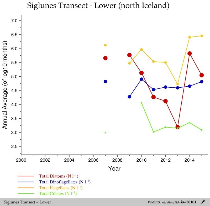
Figure 5: Time-series of annual average of total diatoms, dinoflagellates, flagellates and ciliates from the Siglunes transect (north Iceland). Source: COPEPODITE (http://www.st.nmfs.noaa.gov/copepod/time-series/is-30101/html/zoom-groupsbox.html).
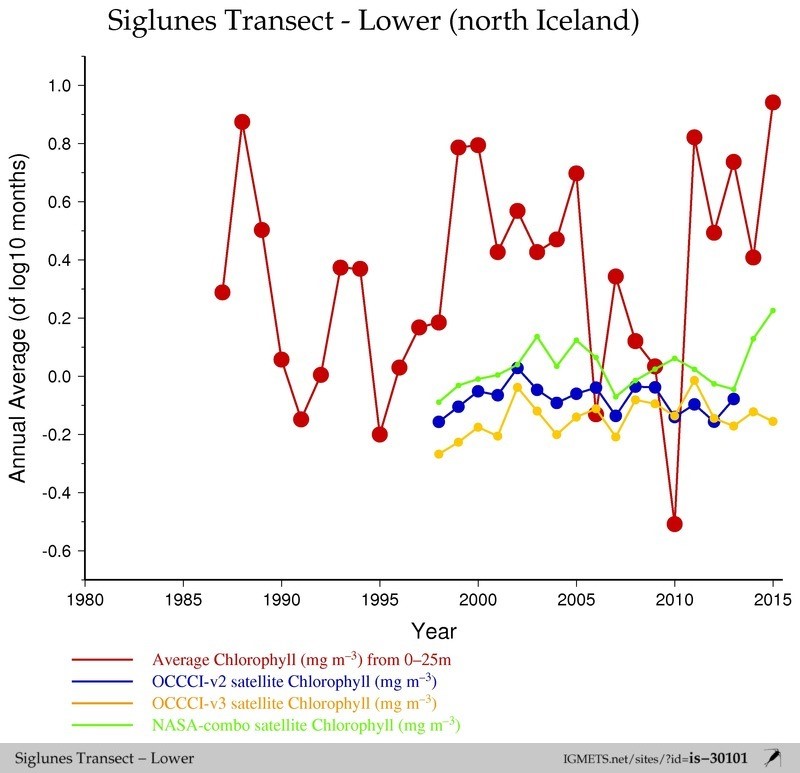
Figure 6: Time-series of annual average of Chlorophyll concentration, measured by four different measuring units, from the Siglunes transect (north Iceland). Source: COPEPODITE (http://www.st.nmfs.noaa.gov/copepod/time-series/is-30101/html/zoom-groupsbox.html).
The Phytoplankton Monitoring Network offers an interactive viewing map, which shows monitoring data on species level (https://www.ncddc.noaa.gov/). However, when searching for all species, only a three month time period can be shown. When only showing data on blooms, all species can be selected. When searching between 2008 and 2017, no monitoring data in the study area (Arctic) or tributary water systems are available.
The Arctic Ocean Diversity website offers Plankton data sets (http://www.arcodiv.org/Database/Plankton_datasets.html). Of these data sets, only one contains phytoplankton: Phytoplankton of the White Sea, Barents Sea, Amundsen & Nansen Basins, 1993-2003. The data can be downloaded as CSV or XML file.
Data use, availability and gaps
Data was available but sparse, in comparison to the breadth of the question asked. However, the lack of data is relatively easy to explain; data gathering is very time and money consuming. The available data is very specific for a certain time and space and averaging does not work well. Data gaps exist in both time and space, especially on species level. More data is available on species groups level or simply on primary production or chlorophyll concentrations, which is easier to measure. Consistent monitoring is needed to create reliable time series.
Conclusion and lessons learned
On a species level, it is difficult and unwise to generalize the most common species in the Arctic area, as the area is simply too large and diverse. Even in smaller areas the most common species differ year to year and season to season. No direct conclusion can be drawn from the assembled data. Lessons learned during the gathering of the data are:
Recommendations
When interested in phytoplankton species composition and change in the entire Arctic area, an extensive monitoring and research program should be set up. This is highly recommended in the fast-changing Arctic area, focused on melting sea-ice and changing upwelling conditions for many species.
Recommendations:
- Pan-Arctic approach on the study of phytoplankton. Set up consistent monitoring programs to better understand the distribution and change in phytoplankton in the Arctic area.
- Create an open sourced phytoplankton datahub for the Arctic area, including data downloads and map availability.
- Focus on the influence of climate change on phytoplankton and translate this into consequences further up the food chain.
- Focus on Ice-edge areas throughout the year to research the phytoplankton community and development.
- Link to alien species and shipping routes, as shipping might be an important factor in bringing alien species of phytoplankton to the Arctic area.
- World-wide or at least Arctic-wide standardisation of monitoring and reporting.
-
References:
- Total Diatoms (#/l) from 2007 to 2015
- Total Dinoflagellates (#/l) from 2007 to 2015
- Total Flagellates (#/l) from 2007 to 2015
- Total Ciliates (#/l) from 2007 to 2015
- Average Chlorophyll (mg/m3) from 0-25m from 1987 to 2015
- Data on phytoplankton is available, but limited in detail, time and space;
- More data is available on species groups than on individual species level;
- More data is available on Chlorophyll concentrations;
- Phytoplankton are strongly linked to climate change.
- The study area is quite broad and is home to many different types of (eco-)systems, which makes it unwise to generalize the three most abundant species of phytoplankton.
- Even in small geographical areas the most abundant species may change year to year, so the most abundant species one year may not be the most abundant species the next year. The length of a time series can be crucial for the outcomes and the conclusions drawn.
- Most studies focus on either zooplankton or primary production in a broad sense, generally focusing on chlorophyll concentrations rather than on individual species.
- The data which is available is quite sporadic both on a temporal and spatial level, is presented in different formats and need different levels of processing.
- There seem to be gaps in both time and space of monitored areas in the arctic when it comes to individual species of phytoplankton. Data found was not always up-to-date.
- There are not many permanent monitoring stations for phytoplankton, a lot of the data comes from research expeditions or cruises. Differences in time and space makes comparison between data sets difficult.
- Pan-Arctic approach on the study of phytoplankton. Set up consistent monitoring programs to better understand the distribution and change in phytoplankton in the Arctic area.
- Create an open sourced phytoplankton datahub for the Arctic area, including data downloads and map availability.
- Focus on the influence of climate change on phytoplankton and translate this into consequences further up the food chain.
- Focus on Ice-edge areas throughout the year to research the phytoplankton community and development.
- Link to alien species and shipping routes, as shipping might be an important factor in bringing alien species of phytoplankton to the Arctic area.
- World-wide or at least Arctic-wide standardisation of monitoring and reporting.
- Arrigo, K. R., & Dijken, G. L. Van. (2015). Continued increases in Arctic Ocean primary production. Progress in Oceanography, 136, 60–70. http://doi.org/10.1016/j.pocean.2015.05.002
- Bopp, L., O. Aumont, P. Cadule, S. Alvain, and M. Gehlen (2005), Response of diatoms distribution to global warming and potential implications: A global model study, Geophys. Res. Lett., 32, L19606, doi:10.1029/2005GL023653 http://onlinelibrary.wiley.com/doi/10.1029/2005GL023653/epdf
- Coupel, P., Ruiz-pino, D., Sicre, M., Chen, J. F., Lee, S. H., Schiffrine, N., … Gascard, J. (2015). The impact of freshening on phytoplankton production in the Pacific Arctic Ocean To. Progress in Oceanography, 131, 113–125. http://doi.org/10.1016/j.pocean.2014.12.003
- Falk-Petersen, S., Pavlov, V., Berge, J., Cottier, F., Kovacs, K. M., & Lydersen, C. (2015). At the rainbow’s end: high productivity fueled by winter upwelling along an Arctic shelf. Polar Biology, 38, 5–11. http://doi.org/10.1007/s00300-014-1482-1
- Frey, K. E., Moore, G. W. K., Cooper, L. W., & Grebmeier, J. M. (2015). Divergent Patterns of Recent Sea Ice Cover across the Bering, Chukchi, and Beaufort Seas of the Pacific Arctic Region. Progress in Oceanography, 136, 32–49. http://doi.org/10.1016/j.pocean.2015.05.009
- Hallegraeff, G. M. (2010). Ocean climate change , phytoplankton community responses, and harmful algal blooms: a formidable predictive challenge. Journal of Phycology, 46, 220–235. http://doi.org/10.1111/j.1529-8817.2010.00815.x
- Hoppe, C. , Schuback, N. , Wolf, K. , Semeniuk, D. , Giesbrecht, K. , Maldonado, M. T. , Varela, D. E. , Rost, B. and Tortell, P. D. (2016): Combined effects of ocean acidification and enhanced irradiances on Arctic phytoplankton assemblages – Why do they not care? , Gordon Research Conference ‘Global Ocean Change Biology’, Waterville Valley, NH, USA, 17 July 2016 - 22 July 2016. http://epic.awi.de/41613/
- Larsen, J. N., Anisimov, O. A., Constable, A., Hollowed, A. B., Maynard, N., Prestrud, P., … Stone, J. M. R. (2014). Polar Regions. In V. R. Bggarros, C. B. Field, D. J. Dokken, M. D. Mastrandrea, K. J. Mach, T. E. Bilir, … L. L. White (Eds.), Climate Change 2014: Impacts, Adaptation, and Vulnerability. Part B: Regional Aspects. Contribution of Working Group II to the Fifth Assessment Report of the Intergovernmental Panel on Climate Change (pp. 1567–1612). Cambridge, United Kingdom and New York, NY, USA: Cambridge University Press.
- Logvinova, C., Frey, K., Mann, P., Stubbins, A., & Spencer, R. (2015). Assessing the potential impacts of declining Arctic sea ice cover on the photochemical degradation of dissolved organic matter in the Chukchi and Beaufort Seas. Journal of Geophysical Research Biogeosciences, 120(11), 2326–2344. Retrieved from http://onlinelibrary.wiley.com/doi/10.1002/2015JG003052/full
- http://earthobservatory.nasa.gov/Features/Phytoplankton/ (Earth Observatory)
- http://www.arcodiv.org/Database/Plankton_datasets.html (Arctic Ocean Diversity)
- https://www.ncddc.noaa.gov/website/PMN/viewer.htm (Phytoplankton Monitoring Network)
- https://www.nodc.noaa.gov/OC5/BARPLANK/WWW/INV_CRUS/inventory.html (Ocean Climate Laboratory)
- http://www.st.nmfs.noaa.gov/copepod/ (COPEPOD)
- http://www.st.nmfs.noaa.gov/copepod/time-series (COPEPODITE)
- https://www.climate.gov/news-features/features/sea-ice-declines-boost-arctic-phytoplankton-productivity (NOAA Climate.gov)
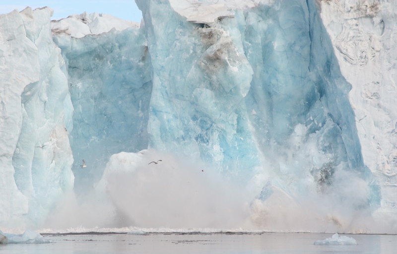
Photo: Martine van den Heuvel-Greve