 Within the Arctic, different types of national Marine Protected Areas (MPAs) have been established under national legislations. The Arctic covers a number of seas under national jurisdictions as well as areas beyond national jurisdictions (high seas). High sea MPAs, known as Vulnerable Marine Ecosystems (VMEs), have been established by Regional Fisheries Management Organisations (RFMOs). In this challenge we present an overview of all these types of MPAs. Additionally, we evaluate the current MPA network in terms of how representative and coherent it is, and how likely MPAs are to be affected by climate change.
Objectives of the challenge
1. Gather data to compile a (geographical) database of the Marine Protected Areas within the Arctic (Phase I)
2. IUCN classification of MPAs (Phase I)
Read more
Summary
In this task, a database of Arctic MPAs was set up based on the World Database of MPAs in combination with a number of other databases. Each MPA was assigned to a IUCN category.
Table 1. IUCN Categories (for details, see the IUCN classification)
| Description | |
| Ia | Strict Nature Reserve |
| Ib | Wilderness area |
| II | National Park |
| III | Natural Monument or feature |
| IV | Habitat/species management area |
| V | Protected landscape/seascape |
| VI | Protected area with sustainable use of natural resources |
| Not Reported | For protected areas where an IUCN category is unknown and/or the data provider has not provided any related information. |
| Not Applicable | The IUCN Management Categories are not applicable to a specific designation type. This currently applies to World Heritage Sites and UNESCO MAB Reserves. |
| Not Applicable also applies to a site that does not fit the standard definition of a protected area (PA_DEF field = 0). | |
| Not Assigned | The protected area meets the standard definition of protected areas (PAF_DEF = 1) but the data provider has chosen not to use the IUCN Protected Area Management Categories. |
Results
IUCN Classification: 492 MPAs were included in the database and classified according to the IUCN classification (Table 1). This includes 57 MPAs that were added during this project . These additional MPAs lacked an IUCN classification (‘blanks’). Classifications were assigned to each new MPA based on their specific characteristics. The classifications assigned were mainly CAT IV (8 OSPAR MPAs), CAT VI (38 NOAA MPAs near Alaska: a lot of fishery measures.) and ‘Not Applicable’ in case of the 11 CBD EBSAs.
In addition, 71 MPAs within the World Database of MPAs had been classified as ‘not applicable’ or ‘not reported’. In this project, we attempted to classify these as well. For example, the UNESCO-MAB Biosphere reserve (one site, covering about 40% of Greenland) was classified as ‘1B’, and the RAMSAR Sites (35 sites) were classified as ‘VI’. World Heritage Sites (4 sites) were classified as ‘IA’ and ‘IB’. A number of different Norwegian sites (15 sites) are still under consideration, and another group is classified under different categories (see individual sites in the map viewer). RAMSAR definitions were consulted to translate to IUCN categories. This was also done for MPAs from other sources.
Of the total number and surface of MPAs, Norway has most areas assigned (206; Table 2), while the total surface of MPAs (km2) is highest for the USA (Figures 3, 4; Table 1). Per data source, most areas were assigned to only one IUCN category (Figures 5, 6; Table 2).
The World Database of MPAs contained eight MPAs that were removed from the 2015 database (one Russian and seven USA). These areas are shown on the map below (Figure 7).
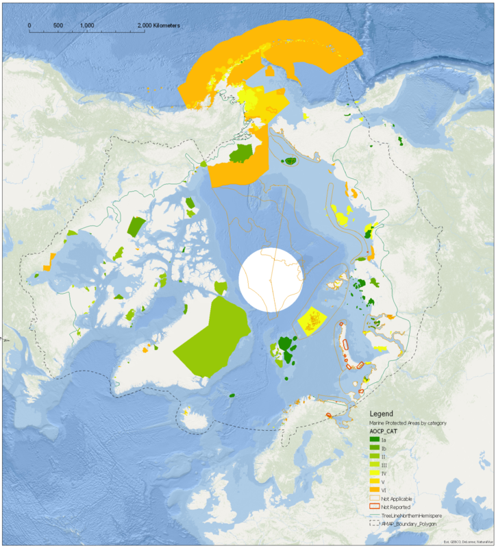
Figure 7. MPAs in the Arctic classified according to the IUCN categories (final results, July 2016). The IUCN categories are: Ia - Strict Nature Reserve, Ib -Wilderness area, II - National Park, III - Natural Monument or feature, IV - Habitat/species management area, V - Protected landscape/seascape, VI -Protected area with sustainable use of natural resources (for details, see the IUCN classification). Not Applicable: the IUCN Management Categories are not applicable to a specific designation type. This currently applies to World Heritage Sites and UNESCO MAB Reserves. Not Applicable also applies to a site that does not fit the standard definition of a protected area (PA_DEF field = 0). Not Reported: For protected areas where an IUCN category is unknown and/or the data provider has not provided any related information.
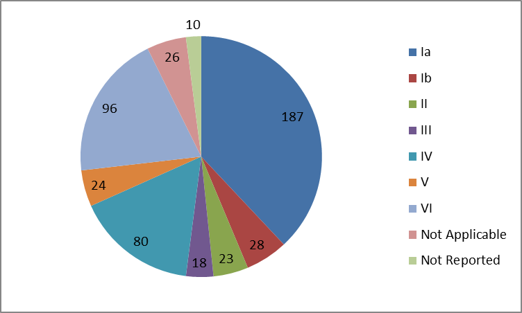
Figure 1. Pie-chart showing number of MPAs per IUCN category.
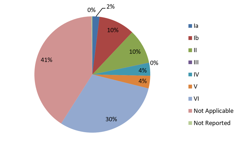
Figure 2. Pie-chart showing coverage % (km2) of MPAs per IUCN category.
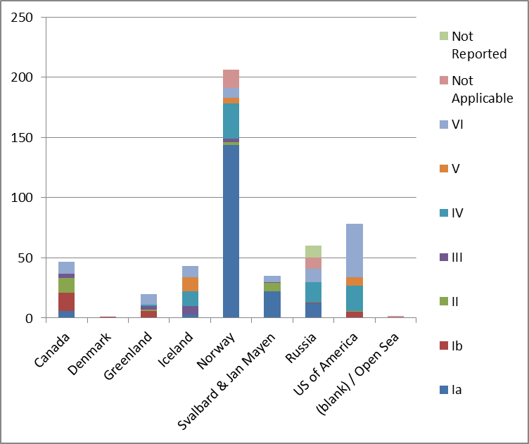
Figure 3. Classification in IUCN categories per region. Y-axis: Number of MPAs, X-axis: countries or regions.
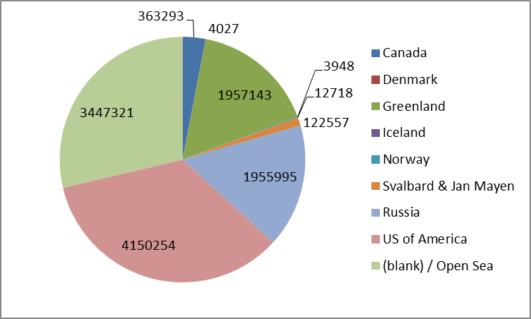
Figure 4. Pie-chart showing surface (km2) covered by MPAs per region.
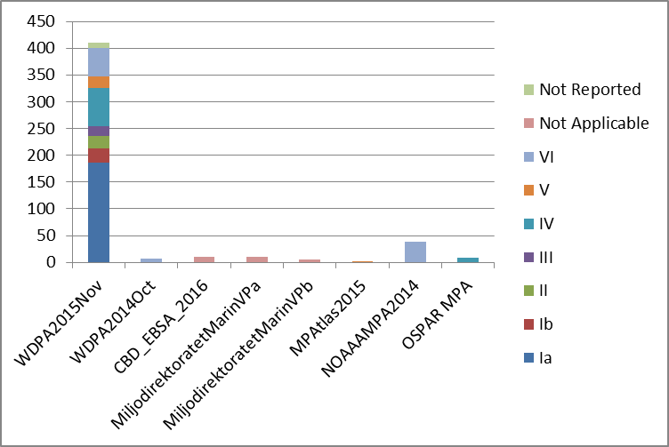
Figure 5. Classification in IUCN categories per source. Y-axis: Number of MPAs, X-axis: data sources.
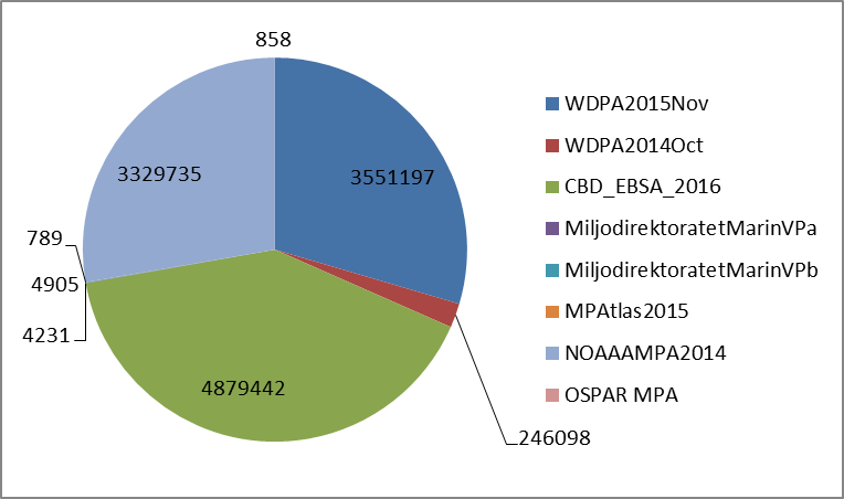
Figure 6. Pie-chart showing surface (km2) covered by MPAs per data source.
Table 2. MPAs per country/region
| IUCN category (reviewed) | ||||||||||
| Country | Ia | Ib | II | III | IV | V | VI | Not Applicable | Not Reported | Grand Total |
| Canada | 6 | 15 | 12 | 4 | 10 | 47 | ||||
| Denmark | 1 | 1 | ||||||||
| Greenland | 6 | 1 | 3 | 1 | 9 | 20 | ||||
| Iceland | 3 | 7 | 12 | 12 | 9 | 43 | ||||
| Norway | 144 | 2 | 3 | 29 | 5 | 8 | 15 | 206 | ||
| Svalbard & Jan Mayen | 22 | 7 | 1 | 5 | 35 | |||||
| Russia | 12 | 1 | 17 | 11 | 9 | 10 | 60 | |||
| US of America | 5 | 1 | 21 | 7 | 44 | 78 | ||||
| Open Sea | 2 | 2 | ||||||||
| Grand Total | 187 | 28 | 23 | 18 | 80 | 24 | 96 | 26 | 10 | 492 |
Table 3. MPAs per source
| IUCN category (reviewed) | ||||||||||
| Source description | Ia | Ib | II | III | IV | V | VI | Not Applicable | Not Reported | Grand Total |
| WDPA2015Nov | 186 | 27 | 23 | 18 | 72 | 22 | 52 | 10 | 410 | |
| WDPA2014Oct* | 1 | 6 | 7 | |||||||
| CBD_EBSA_2016 | 11 | 11 | ||||||||
| MiljodirektoratetMarinVPa | 1 | 10 | 11 | |||||||
| MiljodirektoratetMarinVPb | 5 | 5 | ||||||||
| MPAtlas2015 | 2 | 2 | ||||||||
| NOAA MPA2014 | 38 | 38 | ||||||||
| OSPAR MPA | 8 | 8 | ||||||||
| Grand Total | 187 | 28 | 23 | 18 | 80 | 24 | 96 | 26 | 10 | 492 |
*These MPAs were in not in the WDPA 2015 version, but were included in our database.
References
- WPDA: http://www.protectedplanet.net/
- Norway - Miljødirektoratet.NO http://www.miljodirektoratet.no/no/Tjenester-og-verktoy/Database/ and http://kartkatalog.miljodirektoratet.no/Map_catalog_Dataset_overview.asp
- USA - NOAA: http://marineprotectedareas.noaa.gov/dataanalysis/mpainventory/ Download links: [Date accessed: 20151222]
- Canada - Fisheries and Oceans Canada (DFO)
Webpage with an overview of MPA and Areas of interest [Date accessed: 20151222] - Greenland - Naalakkersuisut = Government of Greenland (website) [Date accessed: 20151222]
http://naalakkersuisut.gl/en/About-government-of-greenland/Travel-activities-in-remote-parts-of-Greenland/Publications has downloads for PDFs for National Parks, Protected Areas and Ramsar Areas. - Iceland - Umhverfisstofnun or Environment Agency of Iceland (http://www.ust.is/the-environment-agency-of-iceland/. [Date accessed: 20151222]
- Russia: Wild Russia [Center for Russion Nature Conservation]. [Date first accessed: 20151222]
- OSPAR MPA Network - http://mpa.ospar.org/home_ospar
- RAMSAR sites - https://www.ramsar.org/sites-countries/
- UNESCO MAB-sites (http://www.unesco.org/new/en/natural-sciences/environment/ecological-sciences/biosphere-reserves/europe-north-america/)
- World Heritage Sites (http://whc.unesco.org/en/list)
- EBSA (Ecologically or Biologically Significant Marine Areas) (https://www.cbd.int/ebsa/about)
3. Produce an analysis of Coherence of the MPA network (Phase II)
Read more
MPA Coherence Data Evaluation (project phase II)
To evaluate the coherence of the MPA network a number of data sets are vital:
- Location of Marine Protected Areas, preferably with associated data on species and habitats.
- Species specific distribution data to be evaluated, preferably with additional information on ecology, habitat preference etc..
We performed a coherence analysis for the Arctic Ocean using a matrix-based approach developed by OSPAR (2006,2008). A more technical description is available in the next section. A geographic database with Marine Protected Areas was collated in phase I of this project. This formed the basis of the coherence analysis. The matrix approach includes bioregions. These were implemented as Large Marine Ecosystem as delineated by PAME (2013). While other checkpoint projects were able to rely fairly heavily on EU-related data portals like EMODnet and Copernicus Marine Environmental Monitoring Service, the scope of these data sources generally excluded the Arctic Ocean. Therefore, the project team in this case had to make the best possible use of other –Arctic specific or global– sources of data.
The main remaining challenge was to source data sets on the species and decide which species to include.
The following data sources were identified and used:
- AquaMaps
- GBIF
- Birds of the World (BirdLife International)
- IUCN Red List
The table below summarises species groups covered by each data source, type of data offered, ease of use and accessibility.
| Description | AquaMaps | GBIF | Birds of the World | IUCN Red List |
| Species groups covered | Sharks and Rays; Bony Fish; Invertebrates and Sea Mammals | Sharks and Rays; Bony Fish; Invertebrates and Sea Mammals; Birds | Birds | Sharks and Rays; Bony Fish; Invertebrates and Sea Mammals; Birds |
| Species groups not covered | Birds | - | Sharks and Rays; Bony Fish; Invertebrates and Sea Mammals | - |
| Type of data offered | Map view; CSV-download (c-squares codes included, offering link to geographic display and analysis) | Map view; species dossier; CSV-download a.o. per species (includes Lon/Lat-coordinates per observation point) | Map view; species dossier; Download on request ESRI File GeoDatabase received | Map view; species dossier; Download on request Shapefile (zipped) received, with additional files |
| Resulting data in GIS | Polygons (vector grid) | Points | Polygons | Polygons |
| Ease of use | Medium | Medium | High | High |
| Data request | Free download | Free download | Required for geographic data. Granted for full data set. | Initial single species request granted, well within stated turnaround times. Second multi-species request unanswered. Also after reminder sent. |
Coherence Analysis
Coherence is an important and desirable characteristic of a network of Marine Protected Areas. A coherent network offers protection to a sufficiently large proportion of species and habitats to ensure their continued survival and existence. It also means that the different elements of the MPA network are within a reasonable distance from each other to support a metapopulation of the species so that migrating or otherwise mobile (e.g. during a larval phase) individuals stand a good chance of reaching a ‘safe haven’ (the next protected area).
To assess the coherence of the MPA network the data set constructed during phase I of the project was used in conjunction with additional data sets on species occurrence and with sea ice as the one major habitat for the Arctic Ocean. For this assessment an evaluation framework developed by OSPAR was used (OSPAR, 2006, 2008). It attempts to assess aspects such as: Adequacy, Viability, and Replication.
The analysis was based on 18 Arctic Bioregions, identical to the Large Marine Ecosystems (LME) as delineated for the Arctic (PAME, 2013)
The second component was the analysis of the population, extent etc. across those 18 bioregions for a 25 species and one habitat (sea ice).
Outcome of the Coherence analysis
While the available data was sufficient to complete the coherence analysis, the process was complicated by the fact that the species data had to be obtained from different sources. This meant that the methodology had to be altered to achieve comparable results.
All species included in the coherence analysis are Arctic species meaning that they make extensive use of the Arctic and are included in Meltofte (2013). From our list the species with the lowest scores for Replication and Adequacy/Viability are bird species that breed in the Arctic, but that are otherwise not very reliant on the Arctic Ocean and Marine Protected Areas.
The least protected Arctic marine mammals are
- the Polar Bear (Ursus maritimus), low Replication score and
- the Hooded Seal (Cystophora cristata), low proportion of the population inside MPA.
MPA Ecological Coherence evaluation
Both the Polar Bear and the Hooded Seal have a strong association with sea ice as an important habitat. Sea ice is also important habitat for the Ringed Seal (Pusa hispida), the Narwhal (Monodon Monoceros), the Ivory Gull (Pagophila eburnea), Polar Cod (Boreogadus saida) and, to a lesser extent the Walrus (Odobenus rosmarus) and Beluga whale (Delphinapterus leucas).
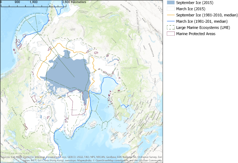
A single habitat has been included in our coherence analysis: sea ice (based on the min. and max. extent recorded in 2015). This habitat has the lowest Replication score within the analysis and also is poorly protected by/represented in current MPA boundaries.
The project team did not find any targets set (internationally or nationally) and focussed on the protection of species and/or habitats in the Arctic Ocean. As a result this column within the matrix was left empty.
All of the results were combined into table 1, with the species/habitat in rows, and the bioregions and other characteristics to be evaluated in columns.
Table 1: MPA Coherence Analysis.
Species/habitat with blue background indicated sea ice and/or a strong association with this habitat. In the columns for the bioregions a light blue background (for mammals, fish and invertebrates) indicates year-round presence within that bioregion. Beluga has a blue outline to indicate a year-round presence in the Arctic (#1). For bird species a slightly darker blue background indicated presence within the bioregion outside the breeding season. For a few bird species bioregions have a blue outline, to indicate presence inside the bioregion outside the breeding region, but with decreased reliance on these bioregions during non-breeding season as the species also make use of large areas outside the Arctic. For Brent Goose, the Hudson Bay has a pale yellow background indicating it is used during migration to/from the breeding grounds in the Arctic and wintering areas further south.
Numbers in the bioregion columns indicate (estimated) population sizes for that region.
Feature targets are part of the OSPAR evaluation framework, however the column remains empty, as no (international) set targets have been identified. The columns for Replication (#2) and Adequacy/Viability (#3)have been colour-coded to aid the interpretation.
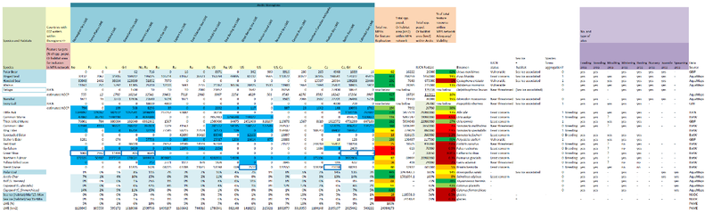
#1: Beluga whales have been evaluated using a data set originating from AquaMaps and within that group it is deviant. Most AquaMap suitability maps have areas where the Overall Probability reaches its maximum value of 1.0. For the Beluga map this is not the case as it peaks at 0.6, and is therefore below the 0.8 threshold used for all other AquaMaps data sets to determine which bioregions are of prime interest to the species.
#2: Colour-coding Replication
| <10 | >10 | >25 | >50 | >100 | >250 |
#3: Colour-coding Adequacy/Viability
| <2.5% | >2.5% | >5% | >10% | >25% | >50% |
The Coherence Analysis has relied on four major sources of information – for the species:
- AquaMaps
- GBIF
- Birds of the World (BirdLife International)
- IUCN Red List
The initial plan was to use the distribution maps that are presented on the IUCN Red List website. Unfortunately, after an initial and rewarded request for Little Auk (Alle alle) a second request did not receive any reply. It may have been that our choice to bundle a dozen or so species into a single request did not fit within the administrative processes at IUCN. It seemed to us that not repeating the same request, with all additional text etc. for each species separately would be more efficient. We also waited for a few weeks –as indicated- before an email was sent to a different address to give notice of not receiving an answer.
AquaMaps was found as an alternative source of data. This data set offers more or less full cover data on occurrence based on an ecological envelope and overall probability of occurrence. The ecological envelope is extracted from amongst others data points from online collection databases such as GBIF and OBIS and includes minimum, optimal and maximum values for such habitat traits as depths, salinity, temperature etc. The resulting data set is available for download as a csv-file and contains a reference to the c-squares system. With proper use of the c-squares information the csv-data can be coupled to the proper polygons thus yielding a geographic data set. Below a sample map is shown for Walrus (Odobenus rosmarus).
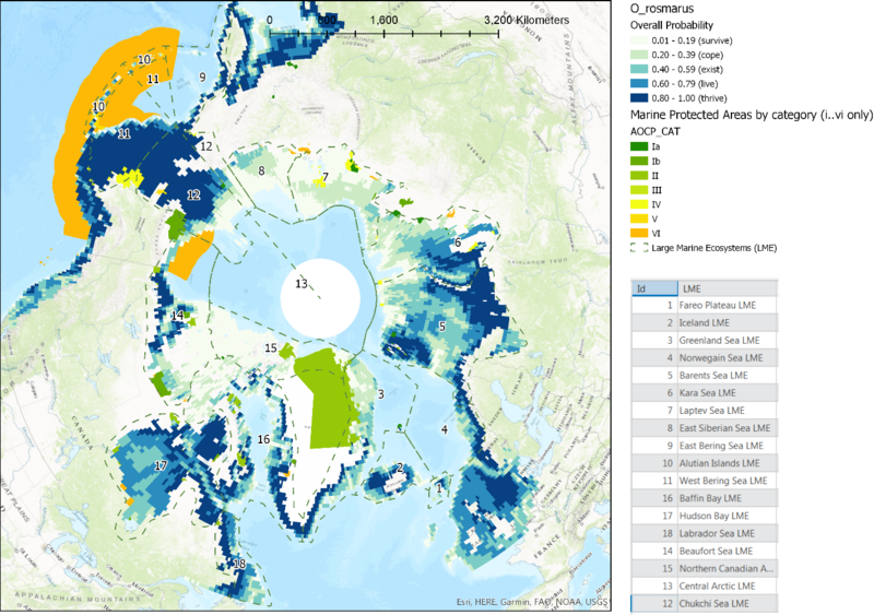
To estimate the population within an LME (bioregion) the summed results of the Overall Probability multiplied by the area of that polygon was used.
AquaMaps (Kaschner et al., 2016) has data for amongst others Sharks and Rays; Bony Fish; Invertebrates and Sea Mammals. No data for birds.
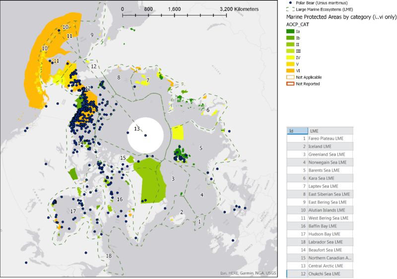
GBIF or in full Global Biodiversity Information Facility was also used. This source provides point data on species occurrence. It has been used for species that were not available from AquaMaps. This data source has been used for one (sea) mammal and two bird species. As an example a map for Polar Bear (Ursus maritimus) is shown.
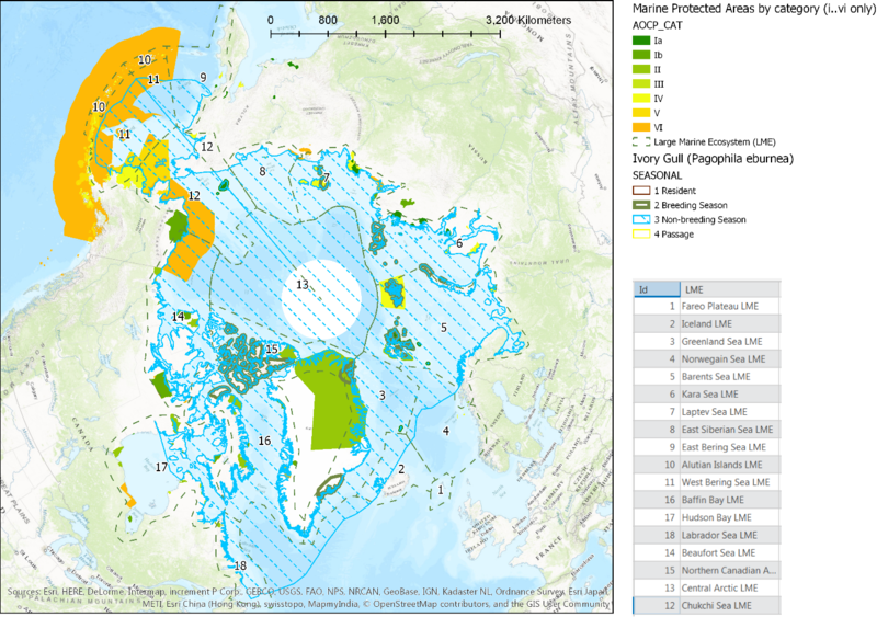
BirdLife International also has much available data, including geographical data sets with polygons for areas used by a species during periods for: 1. resident, 2. breeding, 3. non-breeding, 4. passage and 5. seasonal occurrence uncertain. For consistency the main analysis was based on the breeding season. For most of the bird species that were assessed a large part of the total population breeds strictly within the Arctic (up to 100%) and the habitat is essential. On our request for access to the data BirdLife International replied positively and a copy of the Birds of the World (geodatabase) was made available for the project. The geographical data was also shared with IUCN for amongst others the Red List-website.
Several species had multiple entries in the data (most often two) for some Large Marine Ecosystems (bioregions). By examining the GIS data, the (assumed) underlying cause was identified as separate and adjoining polygons stemming from different origins. To correct the results the affected data sets were aggregated to a single total results per LME. An example is shown for the Ivory Gull (Pagophila eburnea).
Processing the data in GIS
The diverse data sets where collated in GIS, where amongst others the data was analysed.
Most data sets did not arrive with a suitable projection already defined. All data sets were projected to a polar projection: WGS 1984 North Pole LAEA Atlantic (WKID 3574). This ensured that further operations that rely on determining distance or overlap between features would work properly. It was found earlier in the project that the software apparently has difficulty handling polar projections correctly.
The C-squares required to geographically interpret the CSV-files from AquaMaps are available for download (size 0.5 degree lon/lat), from the C-squares website. An Arctic subset was selected and then projected (WKID 3574). After this preparation a join operation was all that was needed to correctly show the species distribution on a map.
To collect the statistics as defined in the OSPAR matrix approach for each species several operations were required to:
- Determine the overlap with LMEs and estimate a population size (or similar) per bioregion (=LME).
- For species that have a considerable presence outside the Arctic LMEs during the evaluated season, as was the case for several bird species, an estimate was also made of the numbers per area in use outside the Arctic LMEs. With this the total Arctic population could be extrapolated from the global number. Population sizes were for the most part taken from information presented on the ‘IUCN Red List’-website, as was the IUCN status (e.g Vulnerable or Near threatened).
- Determine the proportion of the species population that could be considered protected based on an overlap with Marine Protected Areas (Adequacy/Viability). The MPA-database created during Phase I of this project was used for this analysis. The area of overlap was measured for the polygon-based data sets taken from the Bird of the World-database and the AquaMaps-distribution maps. The AquaMaps data has information on how suitable a given c-square is evaluated as and this was used to weigh the area accordingly (highly suitable squares weighted the most). A search distance of 25 km for point data was used so that any observation point up to that distance outside an MPA would still be considered protected. The reasoning behind this was that there is a chance that the observation position is not exact, the observation is subject to coincidence and the species are mobile. Most of the species could, within a fairly short period, reach the relative safety offered by an MPA. Note: the same search distance has also been applied for point data in relation to LMEs.
- Determine the number of MPAs that contribute to the protection of a species (Replication).
References:
- AquaMaps. (2017). http://www.aquamaps.org/
- BirdLife. (2017). Birds of the World, BirdLife International, http://datazone.birdlife.org/home
- c-squares (2016). http://www.cmar.csiro.au/csquares/
- GBIF. (2017). Global Biodiversity Information Facility, http://www.gbif.org/species
- IUCN. (2017) IUCN Red List, http://www.iucnredlist.org/
- Kaschner, K., K. Kesner-Reyes, C. Garilao, J. Rius-Barile, T. Rees, and R. Froese. 2016. AquaMaps: Predicted range maps for aquatic species. World wide web electronic publication, www.aquamaps.org, Version 08/2016.
- Meltofte, H. (2013). Arctic biodiversity assessment. Status and trends in Arctic biodiversity. Akureyri. Retrieved from http://www.abds.is/
- OSPAR. (2006). Guidance on developing an ecologically coherent network of OSPAR marine protected areas.
- OSPAR. (2008). A matrix approach to assessing the ecological coherence of the OSPAR MPA network
- PAME. (2013). Large Marine Ecosystems (LMEs) of the Arctic area. Akureyri. Retrieved from http://www.pame.is/images/03_Projects/EA/EA/PAME_revised_LME_map_with_explanatory_text_15_Aug_2013_-_Vefur.pdf
- Rees, Tony, 2003. "C-squares", a new spatial indexing system and its applicability to the description of oceanographic data sets. Oceanography, vol. 16(1): 11-19. Available online at: http://www.cmar.csiro.au/csquares/csq-Arcticle-Mar03-lowres.pdf.
4. Asses the (potential) impact of Climate Change on MPAs (Phase II)
Read more
The initial plan was to assess the effects of climate change in the Arctic on both abiotic factors (melting ice, freshwater input and acidification) and ecological factors (changes in primary production, shifts in species ranges, species distribution and abundance, loss of habitat, change in migratory patterns, etc.) (Soto, 2001; Roessig et al., 2004) at a high level of detail per MPA (specific species, stressors and their magnitude). Unfortunately, this analysis could not be completed, because:
- MPA information does not include specifics on the species and/or habitats that justify designation as an MPA.
- The challenge on Climate Change, Coast and Riverine Inputs did not uncover relevant and usable data sets that could have been (re-)used for the MPA and Climate Change analysis. Neither did the project team find useful data sets on habitats, other than sea ice, for the MPA Challenge and the Coherence analysis.
With the lack of information available to the project, this challenge could not be completed in its intended fashion.
The Coherence analysis resulted in identification of a single threatened habitat: Sea Ice. Sea ice is an essential habitat for a number of Arctic species and is only to a very small extent included within current MPA boundaries. As the root cause of the threats to sea ice in the Arctic Ocean is Climate Change, designating protected areas will not be helpful in safeguarding this habitat.
According to the results of the susceptibility analysis, sea ice is susceptible to climate change. This indicates that there may also be significant ecological consequences of climate change. Climate change induced impacts on the sea ice habitat, will likely impact the local food webs as various species are dependent on the year-round availability of considerable areas of sea ice including:
- the Polar Bear (Ursus maritimus),
- the Hooded Seal (Cystophora cristata),
- Ringed Seal (Pusa hispida),
- Narwal (Monodon Monoceros),
- Ivory Gull (Pagophila eburnea),
- Polar Cod (Boreogadus saida),
- Walrus (Odobenus rosmarus) and
- Beluga (Delphinapterus leucas),
Sea Ice as a habitat threatened by climate change
The presented map of sea ice extent across the Arctic Ocean has been sourced from NSIDC (Fetterer et al., 2016). The 2015 maximum extent (March) and minimum extent (September) for sea ice extent are clearly much lower than the median extent during the period 1981-2010.
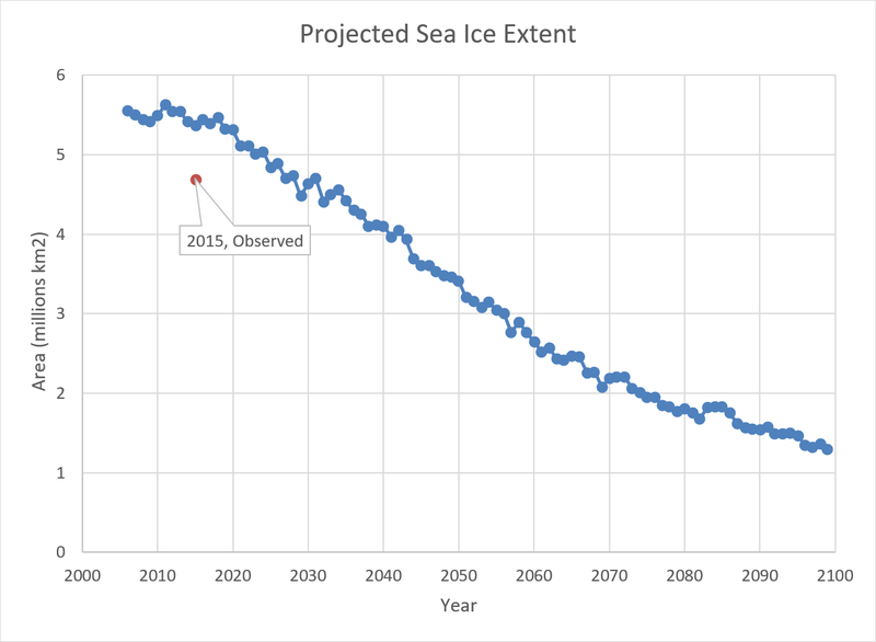
The following graph uses projected data for the minimum extent (September) of Arctic sea ice from 2010 to 2100 (data sourced from One Shared Ocean, 2017), it also includes the (lower) observed sea ice extent for September 2015.
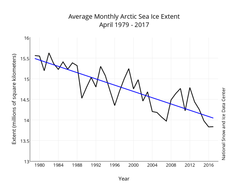
The maximum sea ice extent has also been decreasing (NSICD, 2017) as pictured below. The March 2015 extent as presented above in a map amounts to 14.5 million km2.
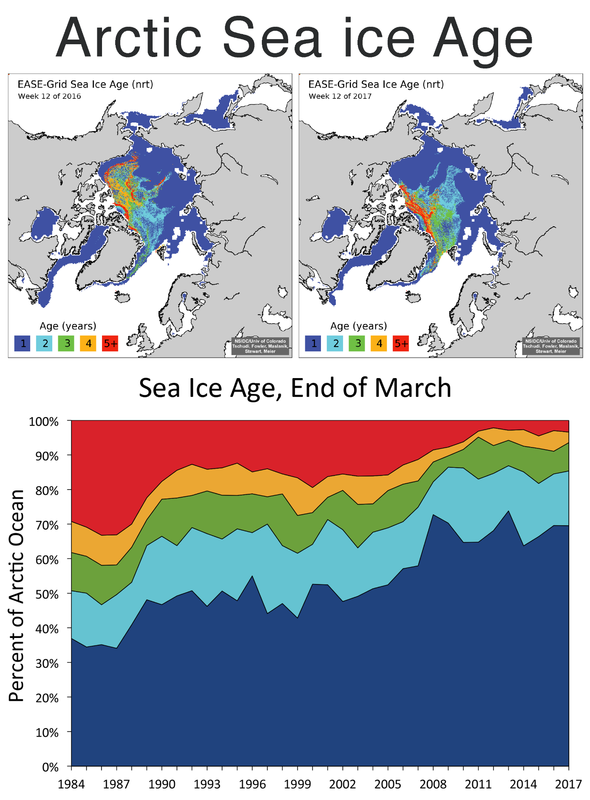
One more characteristic of sea ice that is clearly changing over the last three decades is the amount of multi-year ice, as is illustrated by another graph from NSICD (2017).
References
- Fetterer, F., K. Knowles, W. Meier, and M. Savoie. 2016, updated daily. Sea Ice Index, Version 2. Boulder, Colorado USA. NSIDC: National Snow and Ice Data Center. doi: http://dx.doi.org/10.7265/N5736NV7.
- NSICD. (2017). National Snow and Ice Data Center, News section accessed 5 May 2017, https://nsidc.org/arcticseaicenews/
- One Shared Ocean. (2017). Arctic Sea Ice projection. http://onesharedocean.org/public_store/oo_sea_ice/oo_seaicearctic_rcp85.zip
- Roessig JM, Woodley CM, Cech JJ, Hansen LJ. (2004). Effects of global climate change on marine and estuarine fishes and fisheries. Reviews in Fish Biology and Fisheries 14:251-275
- Soto CG. (2001). The potential impacts of global climate change on marine protected areas. Reviews in Fish Biology and Fisheries 11:181-195
Main results
Arctic MPAs and IUCN classification (Phase I)
In this challenge the network of Arctic MPAs was analysed. Data on MPAs were obtained from various sources, the most comprehensive being the World Database on Marine Protected Areas. In total, 492 marine protected areas were included.
EU Natura 2000 areas or Vulnerable Marine Ecosystems (VMEs) are present in this part of the world. Of the 333 records in the OSPAR database, only eight MPAs were inside the Arctic region, and these were included in the analysis. In total, 11 Norwegian MPAs and five proposed Norwegian MPAs were included. For the USA, 38 additional MPAs published by NOAA were included, including a lot of fishery closures. The network of EBSAs was also included (see Figure 1). An inspection of Greenland, Russian and Canadian (from DFO) data sources did not reveal any MPAs not listed in the Word database.
The resulting data set of MPAs is available in the geoviewer. The geoviewer will also allow for comparisons of the MPA network with habitat maps and fishery intensities.

Figure 1. MPAs in the Arctic classified according to the IUCN categories (final results, July 2016). The IUCN categories are: Ia - Strict Nature Reserve, Ib -Wilderness area, II - National Park, III - Natural Monument or feature, IV - Habitat/species management area, V - Protected landscape/seascape, VI -Protected area with sustainable use of natural resources (for details, see the IUCN classification). Not Applicable: the IUCN Management Categories are not applicable to a specific designation type. This currently applies to World Heritage Sites and UNESCO MAB Reserves. Not Applicable also applies to a site that does not fit the standard definition of a protected area (PA_DEF field = 0). Not Reported: for protected areas where an IUCN category is unknown and/or the data provider has not provided any related information.
Analysis of Coherence of the MPA network (Phase II)
MPA information does not include specifics on the species and/or habitats that justify designation as an MPA and does not present specific species that are protected by the MPA. A selection of species was therefore made to further study the coherence of MPA networks. While the available data was sufficient to complete the coherence analysis, the process was complicated by the fact that the species data had to be obtained from different sources. This meant that the methodology had to be altered to achieve comparable results.
The Coherence analysis resulted in identification of a single threatened habitat: Sea ice. Sea ice is an essential habitat for a number of Arctic species and is only to a very small extent included within current MPA boundaries.
The (potential) impact of Climate Change on MPAs (Phase III)
The initial plan was to assess the effects of climate change in the Arctic on both abiotic factors (melting ice, fresh water input and acidification) and ecological factors (changes in primary production, shifts in species ranges, species distribution and abundance, loss of habitat, change in migratory patterns, etc.) (Soto, 2001; Roessig et al., 2004) at a high level of detail per MPA (specific species, stressors and their magnitude). Unfortunately, this analysis could not be completed, because:
With the lack of information available to the project, this challenge could not be completed in its intended fashion.
The outcome of the Coherence analysis is that sea ice is a threatened habitat within the Arctic and one that is clearly negatively impacted by Climate Change.
Problems and gaps
- Data availability: the IUCN offers data on species distribution on their website. While we made multiple requests for 14 sets of distribution data for analysis within Task 3, we received no reply.
- Language problems: information on Russian MPAs was available on multiple websites, so that by compiling different texts we could form an impression of the status of the MPAs. Texts in most Scandinavian were translatable and for a lot of areas information in English was available as well.
Lessons learned
- The World Database on Protected Areas contained 90% of the MPAs, but is not complete.
- We think the current MPA database developed in this project is relatively complete.
- Geographical Information Systems (GIS): maps need to be projected to a polar projection, because otherwise select-by-location operations give unexpected results. For example, when searching for an area 50 km away from a certain point, a non-polar projection gives incorrect results otherwise.
References
- WPDA: http://www.protectedplanet.net
- Norway - Miljødirektoratet.NO http://www.miljodirektoratet.no/no/Tjenester-og-verktoy/Database/ and http://kartkatalog.miljodirektoratet.no/Map_catalog_Dataset_overview.asp
- USA - NOAA: http://marineprotectedareas.noaa.gov/dataanalysis/mpainventory/ Download links: [Date accessed: 20151222]
- Canada - Fisheries and Oceans Canada (DFO)
- Webpage with an overview of MPA and Areas of interest [Date accessed: 20151222]
- Greenland - Naalakkersuisut = Government of Greenland (website) [Date accessed: 20151222] http://naalakkersuisut.gl/en/About-government-of-greenland/Travel-activities-in-remote-parts-of-Greenland/Publications has downloads for PDFs for National Parks, Protected Areas and Ramsar Areas.
- Iceland - Umhverfisstofnun or Environment Agency of Iceland (http://www.ust.is/the-environment-agency-of-iceland/. [Date accessed: 20151222]
- Russia: Wild Russia [Center for Russion Nature Conservation]. [Date first accessed: 20151222]
- OSPAR MPA Network - http://mpa.ospar.org/home_ospar
- RAMSAR sites - http://www.ramsar.org/sites-countries/the-ramsar-sites
- UNESCO MAB-sites (http://www.unesco.org/new/en/natural-sciences/environment/ecological-sciences/biosphere-reserves/europe-north-america/)
- World Heritage Sites (http://whc.unesco.org/en/list)
- EBSA (Ecologically or Biologically Significant Marine Areas) (https://www.cbd.int/ebsa/about)